Recommender Systems 101 (1) Introduction to Recommender Systems | Xinhe Liu (Charles)

• Modern Recommender Systems
• Recommender System Architecture
• Retrieval Module (Recall)
  • Pre-ranking Module (Coarse Ranking)
  • Fine Ranking
  • Re-ranking / Blending
  • Data Layer
  • Evaluation of Recommender Systems
• Reference

History of Recommender Systems

A recommender system is an information filtering system that predicts user “ratings” or “preferences” for items.

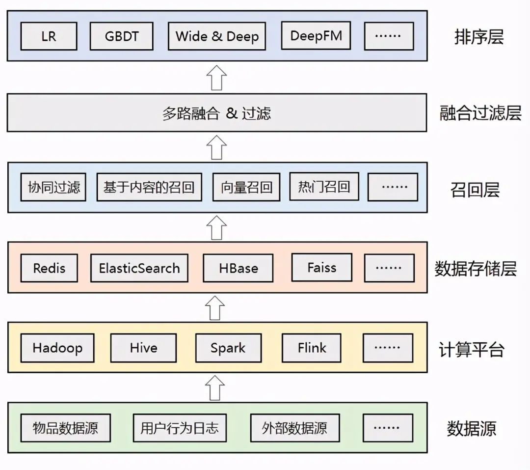
A common recommender system architecture:

• Goal: Match users with information.
• Retrieval (Recall): Guess what content the user might like.
• Ranking: Determine what the user likes most.
• Re-ranking: Apply diversity controls, deduplicate close items, etc.
• Application Scenario: Feed streams, recommendation cards, etc.

flowchart LR subgraph "Recommendation Technical Framework" direction LR A1["Touchpoints"] --> B1["User Features"] A2["User Info"] --> B1 A3["Item Formatting"] --> B2["Item Features"] B1 --> C["Retrieval (Recall)"] B2 --> C C --> D["Ranking"] D --> E["Re-ranking"] E --> F["Application Scenario"] end

History of Recommender Systems:

1. Early Phase (Early 1990s): Originated from library sciences, based on keyword matching and filtering. Key services: early library retrieval systems, academic paper recommendation systems.
2. Collaborative Filtering Era (Late 1990s to Early 2000s): Introduced Collaborative Filtering algorithms, analyzing user behaviors to find similar users or items. Key systems: Amazon’s product recommendations, Netflix’s movie recommendations, Last.fm’s music recommendations.
3. Content-based Filtering Era (Mid-2000s): Based on matching item features with user preferences. Uses metadata and profiles. Key systems: Google News recommendations, Pandora’s music recommendations, StumbleUpon’s web page recommendations.
4. Hybrid Recommendation Era (Late 2000s to Present): Combining Collaborative Filtering and Content-based Filtering to yield more accurate and diverse results. Key systems: Taobao’s product recommendations, Spotify’s music recommendations, LinkedIn’s job recommendations.
5. Personalized Feed Era (Early 2010s): Spearheaded by Toutiao, achieving “one thousand people, one thousand faces” using machine learning. The algorithms became industry benchmarks, driving widespread adoption of personalized feeds.
6. Deep Learning Era (Mid-2010s to Present): Utilizing deep learning to extract rich features, incorporating user behavior sequences and contextual information. Key systems: YouTube’s video recommendations, TikTok’s short video recommendations, Instagram’s content recommendations.
7. Cloud & SaaS Era (2020s to Present): Recommendation algorithms have become standardized cloud services available via APIs. Key services: AWS Personalize, Google Recommendations AI, Azure Personalizer. These package common algorithms (CF, content-based, hybrid) while protecting user privacy.

Collaborative Filtering Algorithms

Collaborative Filtering (CF) is a foundational algorithm in recommender systems. It operates on user behavior data to recommend items and has had a profound impact. CF established the core concept of utilizing user interaction histories, laying the theoretical foundation for matrix factorization, factorization machines (FM), and deep learning recommendation models. The User-Item interaction matrix became the standard way to organize recommendation data, and CF’s approaches to handling sparsity and cold start inspired hybrid and multimodal recommendation methods. Modern systems like YouTube’s deep neural networks and TikTok’s multi-objective recommendations still carry the legacy of CF.

Most standardized recommendation services today (such as Volcano Engine) are heavily built upon collaborative filtering principles.

There are three main types of Collaborative Filtering:

1. Content-based Recommendation: If a user consumes an item of a certain category, recommend other items within that category. For example, recommending other movies starring the same actor.
2. User-based Collaborative Filtering: Operates on the principle that “if a user has similar tastes to a group of people, they will likely enjoy items that those people like.” It finds similar users based on interaction history and recommends items they liked that the target user has not yet seen. For example: “Users who bought this also bought…”
3. Item-based Collaborative Filtering: Operates on the principle that “users are likely to enjoy items similar to what they have liked in the past.” It analyzes item similarities based on user interaction co-occurrences and recommends items similar to the user’s highly-rated items. For example, recommending accessory products that are often purchased together with a main product.

Modern Recommender Systems

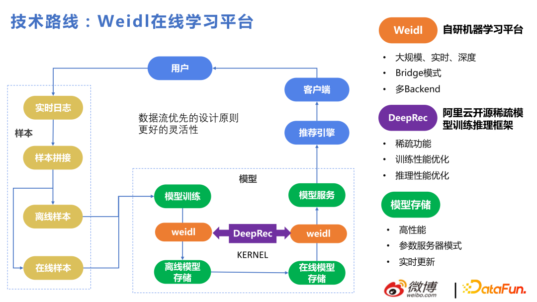
Modern recommender systems follow a data-stream-first design principle, providing high flexibility.

The core workflow is:

1. Collect user behavior data
2. Join training samples
3. Train models
4. Generate recommendations
5. Collect user feedback
6. Update models

This design supports real-time, near-instant updates, featuring:

1. Model Training & Deployment
   • Supports multiple training frameworks: LR (Logistic Regression), FM (Factorization Machines), TensorFlow, DeepRec, etc.
   • Proprietary model storage: Unified data stream architecture and model formats.
   • Quick updates: The pipeline from model training to online serving completes in minutes.
   • Multi-backend support: Flexible switching between different computing backends.
2. Platformized Development
   • Compatible with standard operators from deep learning frameworks and proprietary optimized operators.
   • Supports custom operator development.
   • Performance tuning: Memory allocation and operator optimizations tailored for specific frameworks.
   • Framework migration: Migrated from TensorFlow to DeepRec in 2022, confirming that performance optimization ideas are highly portable.

This architecture ensures recommender systems can respond rapidly to business needs while maintaining a flexible tech stack.

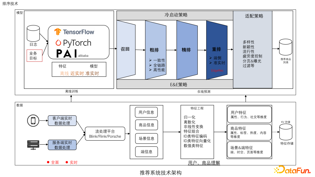
Recommender System Architecture

Retrieval Module (Recall)

The goal of the retrieval module is to quickly filter out candidate subsets related to user interests from the massive candidate pool, achieving high recall at low computational costs. Main features:

1. Efficiency First: Processes millions or billions of candidates, requiring highly efficient algorithms.
2. Wide Coverage: Ensures that potentially relevant content is not missed, chasing high recall.
3. Diversity: Employs multi-channel retrieval strategies to guarantee content diversity.
4. Real-time: Rapidly responds to the user’s latest behaviors and interest shifts.

Engineering implementation: Typically uses multi-channel retrieval followed by merging/fusion.

1. Combine user, item, and behavioral features to fetch candidates from various channels.
2. Utilize vector search and indexing technologies for efficient online retrieval.
3. Merge results from multiple channels to balance efficiency and diversity.

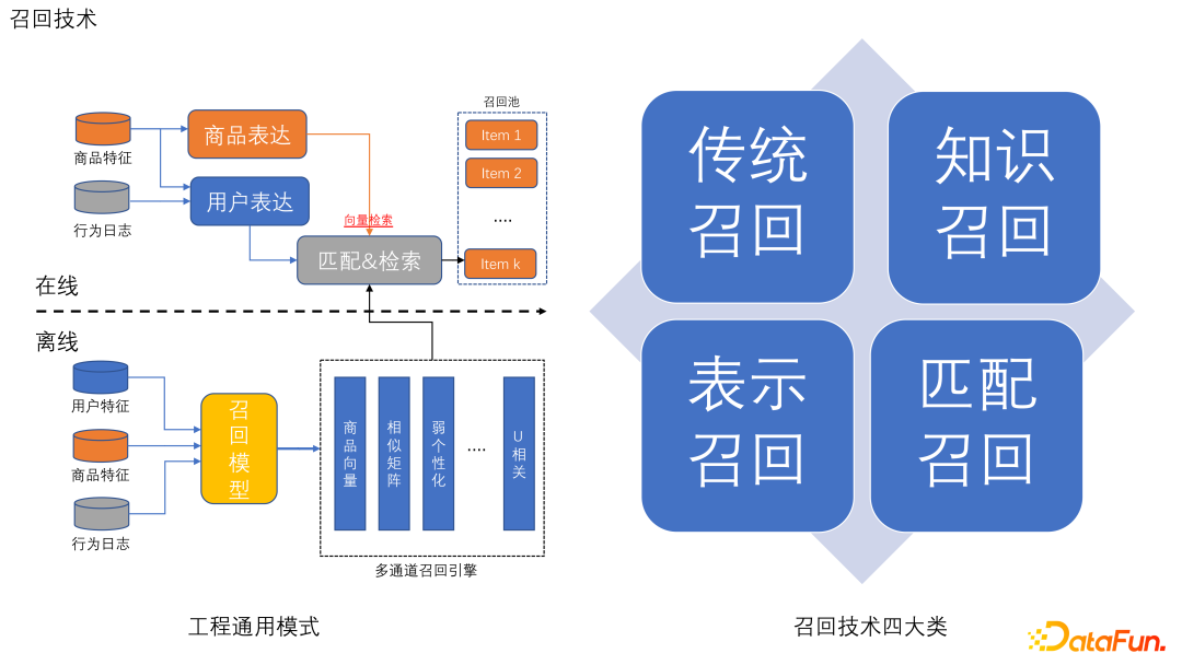
Common Retrieval Strategies: Retrieval techniques can be classified into four main categories: traditional, knowledge-based, representation-based, and matching-based. In practice, these methods are often blended.

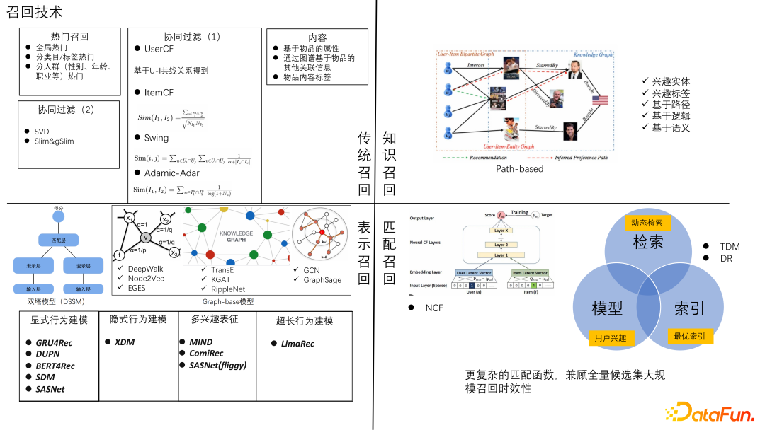
1. Traditional Retrieval
   • Although its usage has decreased in recent years, it still holds a vital position.
   • Includes popularity-based retrieval, collaborative filtering retrieval, and content-based retrieval.
     • Collaborative Filtering: Based on user behavior similarity.
     • Content-based: Matching item attributes and user tags.
     • Popularity/Recency: Based on global popularity and fresh content.
   • Representative algorithms: SVD, Slim series (gSlim, fSlim), UserCF, ItemCF, Swing, etc.
2. Knowledge-based Retrieval
   • Built on knowledge graphs, featuring high interpretability and performance.
   • Implementation: Constructed via graphs or hard rules.
     • Social network retrieval: Based on user social graphs.
     • Explicit interest tags: Based on user selected interests.
   • Applications: Entity-based, tag-based, path-based reasoning, and logical expression matching.
3. Representation-based Retrieval
   • Vector search retrieval (mapping users and items into the same vector embedding space).
   • Evolved from simple dual-tower (two-tower) models to complex graph-based models.
   • Key categories:
     • Explicit behavior modeling:
       • GRU4Rec (Gated Recurrent Units for Recommendation)
       • DUPN (Deep User Perception Network)
       • BERT4Rec (Bidirectional Encoder Representations from Transformers for Recommendation)
     • Implicit behavior modeling:
       • XDM (eXtreme Deep Factorization Machine)
     • Multi-interest representation:
       • MIND (Multi-Interest Network with Dynamic routing)
       • SASNet (Self-Attention Sequential Network)
     • Ultra-long sequence modeling
4. Matching-based Retrieval
   • Uses higher model complexity to achieve precise behavior representation.
   • Representative algorithms:
     • NCF (Neural Collaborative Filtering)
     • TDM (Tree-based Deep Matching)
     • DR (Deep Retrieval)
   • TDM and DR optimize retrieval pipelines across indexing, modeling, and searching.
   • Requires precise negative sampling strategies.

Pre-ranking Module (Coarse Ranking)

The goal of the pre-ranking module is to perform a more refined scoring on the candidates filtered out during retrieval, bridging the gap between retrieval and ranking.

Pre-ranking balances model complexity and computational efficiency, processing hundreds to thousands of candidates and outputting the top subset for the fine ranking stage. Main features:

1. Accuracy-Efficiency Balance: More accurate than retrieval, more efficient than fine ranking.
2. Feature Utilization: Uses a richer feature set than retrieval, but much more streamlined than fine ranking.
3. Model Complexity: Medium complexity, typically using lightweight deep learning models.
4. Candidate Scale: Processes hundreds to thousands of candidates, outputting dozens to hundreds of results.

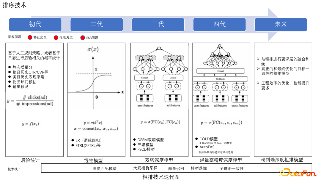
Evolution of Pre-ranking:

• Early Phase: Based on manual rules or posterior probabilities—simple but limited in expressive power.
• Mid-term Phase: Introduced lightweight linear models like LR, XFTRL, and GBDT, providing basic feature representation.
• Modern Phase: Lightweight deep learning models (such as two-tower, three-tower, and FSCD models) that represent users and items separately before matching them, significantly improving expressive power.
• Latest Trends: End-to-end deep pre-ranking, co-optimizing with the fine ranking model.
  • Models like COLD and AutoFAS optimize features and model structures to chase higher accuracy.
  • Model Distillation: Using knowledge distillation so the pre-ranking model learns the capabilities of the fine ranking model, maintaining decision consistency.
  • Objective Alignment: Aligning the pre-ranking objective with the overall system objectives.
  • Engineering Efficiency: Optimizing inference speeds to handle increasing model complexity in real-time.

Key Challenges in Pre-ranking:

1. Maintaining consistency between retrieval, pre-ranking, and fine ranking.
2. Enhancing model representation within tight computing budgets.
   • Feature interaction design: achieving effective feature interaction in lightweight models.
   • Inference-accuracy tradeoffs: boosting accuracy without violating online latency bounds.
   • Sample Selection Bias (SSB): Mitigating data distribution shifts caused by filtering in earlier stages.

Fine Ranking

The fine ranking module is the core sorting layer. It scores the candidates output by the pre-ranking stage, directly determining the quality of the final recommendation list. Main features:

1. High Precision First: Prioritizes predictive accuracy; it is the core decision node.
2. Rich Features: Employs the most comprehensive feature set, including user, item, context, and cross features.
3. High Model Complexity: Employs complex deep learning architectures to capture non-linear relationships.
4. Candidate Scale: Processes dozens to hundreds of candidates, outputting the final sorted list.

Core Objectives of Fine Ranking:

1. Accurate User Behavior Prediction: Accurately predicting CTR, CVR, and other key user interaction probabilities.
2. Multi-objective Balance: Jointly optimizing click-through rate, conversion rate, stay time, and user experience.
3. Real-time Responsiveness: Executing complex model inferences within strict latency budgets.
4. Explainability: Generating explanations for recommendations to build user trust.

Evolution of Fine Ranking Models:

1. Traditional Machine Learning Phase
   • Linear Models: LR (Logistic Regression), MLR (Mixed Logistic Regression).
   • Tree Models: GBDT (Gradient Boosting Decision Tree), XGBoost.
   • Factorization: FM (Factorization Machines), FFM (Field-aware Factorization Machines).
   • Implementations: Using MLR for subgroup modeling, FM for feature interactions, and GBDT/XGBoost for sequence processing. Used FTRL/XFTRL for online learning.
   • Pros: High training and inference efficiency, strong interpretability.
   • Cons: Limited representation power; struggles to capture high-order feature interactions.
2. Early Deep Learning Phase
   • Foundational Deep Networks: DNN (Deep Neural Network), Wide & Deep.
   • Enhanced Feature Interactions: DeepFM, DCN (Deep & Cross Network), xDeepFM.
   • Pros: Automated high-order feature interactions; boosted model expressive power.
   • Cons: Insufficient modeling for user sequence and temporal dynamics.
3. Attention Mechanism Phase
   • Behavior Sequence Modeling: DIN (Deep Interest Network), DIEN (Deep Interest Evolution Network).
   • Multi-interest Modeling: MIND (Multi-Interest Network), ComiRec.
   • Pros: Captures dynamic shifts in user interests, boosting personalization.
   • Representative Models:
     • DIN: Weights history items using an attention mechanism, highlighting historical behaviors relevant to the candidate item.
     • DIEN: Introduces an interest evolution network on top of DIN to model the dynamic shifts in user interests over time.
     • SIM (Search Interest Model): Blends search and browsing history to capture comprehensive user interest.
4. Multi-Task Learning Phase
   • Shared Representation Learning: Shared-Bottom, MMoE (Multi-gate Mixture-of-Experts).
   • Task Relationship Modeling: PLE (Progressive Layered Extraction), Adaptive Information Transfer Multi-task (AITM).
   • Pros: Jointly optimizes multiple business objectives, boosting overall performance.
   • Representative Models:
     • MMoE: Shares bottom expert networks and designs separate gating networks for each task to balance sharing and specialization.
     • PLE: Utilizes layered extraction to decouple task-specific and shared expert networks, addressing negative transfer.
5. Pre-training & Transfer Learning Phase
   • Large-scale Pre-training: BERT4Rec, P5 (Personalized Prompt Learning for Product Search).
   • Cross-domain Transfer: STAR (Sparse Transfer Learning for Recommendation).
   • Pros: Leverages massive datasets and cross-domain knowledge to solve cold-start and data sparsity.
   • Cons: High computing requirements; complex engineering infrastructure.

Core Challenges in Fine Ranking:

1. Multi-objective Optimization: Balancing click-through rates, conversion rates, and user retention.
   • Solutions: Multi-task learning, Pareto efficiency, constrained optimization.
2. Sample Bias Mitigation: Dealing with selection bias, position bias, and exposure bias.
   • Solutions: Counterfactual learning, causal inference, debiasing techniques.
3. Cold Start: Recommending new items or serving new users with sparse data.
   • Solutions: Meta-learning, transfer learning, content feature enhancement.
4. Computational Efficiency: Serving complex model inferences in milliseconds.
   • Solutions: Model compression, knowledge distillation, distributed computing.
5. Explainability: Generating clear reasons for recommendations.
   • Solutions: Attention visualization, feature importance analysis, local surrogate models.

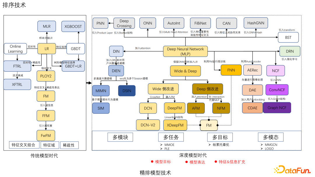
The evolution diagram can be divided into four tracks:

• Bottom Track: MLP to Wide & Deep evolution line, including Deep & Cross Network (DCN), DeepFM, Attentional Factorization Machine (AFM), and Neural Factorization Machine (NFM), optimizing specific structures.
• Top Track: Enhancements to the MLP architecture, introducing Attention, Product Layers, and Graph Neural Networks (GNN).
• Right Track: Variations and improvements based on Autoencoders (AE), Reinforcement Learning, and Neural Collaborative Filtering (NCF).
• Left Track: Attention-based sequence models, including Deep Interest Network (DIN), Deep Interest Evolution Network (DIEN), Multi-channel Interest Merge Network (MIMN), Deep Session Interest Network (DSIN), and Search Interest Model (SIM), focusing on long-sequence modeling.

Fine ranking models are heading towards multi-module, multi-task, multi-objective, and multi-modal integration.

Re-ranking / Blending

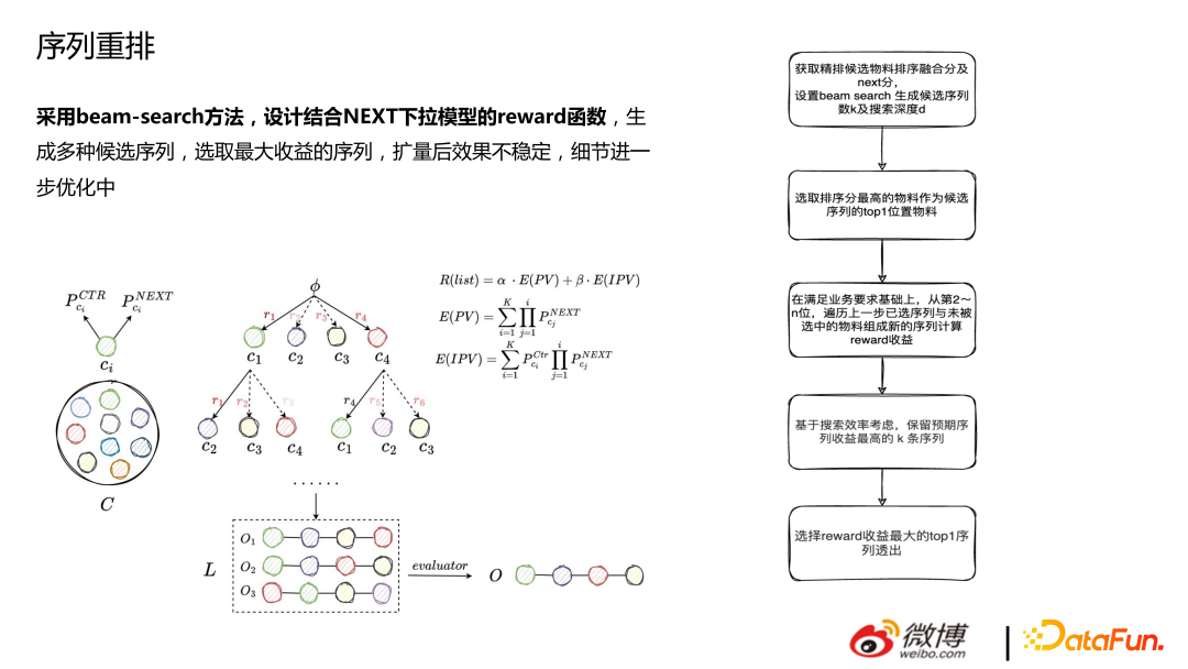
Re-ranking is the final stage. It adjusts and optimizes the candidate list output by the fine ranking stage to maximize overall platform metrics. Unlike fine ranking, re-ranking handles:

1. Global Optimization: Considering the diversity, novelty, and coverage of the list as a whole.
   • Solutions: Greedy algorithms, Integer Programming, Reinforcement Learning.
2. Context Awareness: Factoring in the user’s current session state, past interactions, and visual layout constraints.
   • Solutions: Sequence models, attention mechanisms, graph neural networks.
3. Real-time Feedback: Adapting rapidly based on the user’s immediate feedback signals.
   • Solutions: Online learning, incremental updates, edge computing.

Re-ranking Approaches:

1. Rule-based Re-ranking
   • Diversity Rules: Limiting the proportion of identical categories, scattering similar items.
   • Constrained Rules: Business rules, compliance filters, editorial controls.
   • Pros: Strong interpretability; easy to implement and adjust.
   • Cons: Struggles to capture complex, dynamic patterns; high maintenance cost.
2. Model-based Re-ranking
   • Global Listwise Models: DLCM (Deep Listwise Context Model), PRM (Personalized Re-ranking Model).
   • Sequence-aware Models: SetRank, Intent-aware Re-ranking with Graph Neural Networks (IRGPR).
   • Pros: Learns global dependencies across the candidate list, boosting list quality.
   • Cons: High computational complexity under tight latency budgets.
3. Reinforcement Learning-based Re-ranking
   • Policy Gradient: REINFORCE, Actor-Critic.
   • Value-based: DQN, Double DQN.
   • Pros: Directly optimizes long-term rewards; handles delayed feedback.
   • Cons: Unstable training; low sample efficiency.
4. Edge Computing Re-ranking
   • Lightweight Models: EdgeRec (Alibaba), MobileRec.
   • Model Compression: Quantization, pruning, knowledge distillation.
   • Pros: Ultra-low latency; leverages real-time on-device signals.
   • Cons: Limited computational capacity on client devices.

Re-ranking Challenges:

1. Latency Constraints: Running complex global listwise optimizations in milliseconds.
   • Solutions: Model compression, calculation optimization, distributed processing.
2. Metric Multiplicity: Balancing conversions, diversity, and long-term user satisfaction.
   • Solutions: Multi-objective optimization, weighted scoring, A/B testing.
3. Exploration vs. Exploitation: Introducing exploration mechanisms to prevent recommendation feedback loops.
   • Solutions: Thompson sampling, contextual multi-armed bandits.
4. Fairness: Ensuring content diversity and algorithmic fairness.
   • Solutions: Fairness constraints, audit checks.

Data Layer

The data layer is the foundation, collecting, processing, and storing data to support upstream algorithms. A mature data layer contains:

1. Data Collection System
   • Event tracking design, collection protocols, and pipelines.
   • User behavior data: Clicks, impressions, stay time, favorites, shares, comments, etc.
   • Content features: Structured and unstructured features for text, images, video, and audio.
   • Contextual data: Time, location, device, network conditions, etc.
   • Transactional data: Purchases, payments, refunds, customer support, etc.
2. Data Processing Framework
   • Real-time: Kafka, Flink, Spark Streaming, etc.
   • Offline: Hadoop, Spark, Hive, etc.
   • Feature Storage: Redis, HBase, Cassandra, Feature Store (e.g., Alibaba’s FeatureStore).
3. Feature Engineering System
   • Extraction: Extracting high-value signals from raw logs.
   • Transformation: Normalization, standardization, bucketization, encoding, etc.
   • Selection: Filtering, embedding, wrapper methods.
   • Crossing: Cross-features, multi-domain feature fusion.
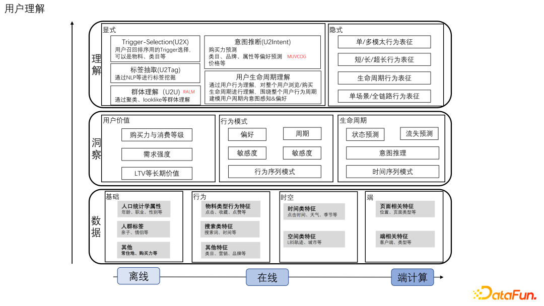
4. User Understanding System
   • Data Layer: Collecting user demographics, behaviors, contexts, and device logs. Requires robust real-time tracking.
   • Insight Layer: Deep analysis of user characteristics (LTV, churn risk, purchase cycles, interest shifts, user lifecycle stage).
   • Understanding Layer:
     • Explicit: Extracting interest tags, category preferences, and user clusters (Lookalike models).
     • Implicit: Vectorizing user histories, modeling sequence patterns across short, long, and ultra-long lifecycles.
   • Explainability: Generating recommendation reasons based on user/item similarities and social graphs.

Key Challenges:

1. Data Quality: Ensuring completeness, accuracy, and fresh, latency-free updates.
2. Scale: Storing petabytes of historical logs and supporting millions of QPS under millisecond read latencies.
3. Privacy: Data masking, access control, and compliance with GDPR, CCPA, etc.

Evaluation of Recommender Systems

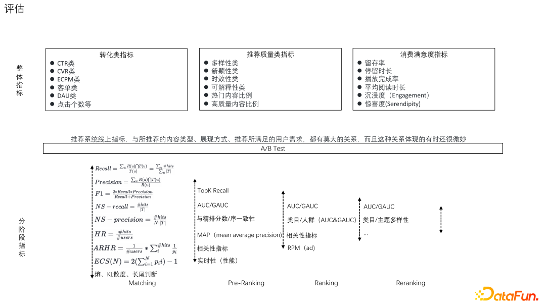
Evaluation ensures system efficacy and guides iterative optimization, split into online business metrics and离线 model metrics:

Online / Business Metrics

Directly measures real-world impact and platform value:

1. Conversion Metrics
   • Click-Through Rate (CTR): Proportion of recommendations clicked.
   • Conversion Rate (CVR): Proportion of clicks resulting in conversion.
   • Order Rate: Proportion of sessions resulting in orders.
   • Retention Rate: The long-term retention impact of recommendations.
2. Recommendation Quality
   • Coverage: The proportion of unique items recommended out of the total catalog.
   • Diversity: Category richness across the recommendation list.
   • Novelty: The proportion of fresh/unseen items recommended.
   • Relevance: The degree of match with the user’s active interests.
   • Recency/Timeliness: Real-time update capacity.
3. User Satisfaction
   • User Ratings: Direct explicit feedback.
   • Dwell/Stay Time: Dwell duration on recommended content.
   • Interaction Depth: Deep interactions like shares, comments, favorites.
   • NPS (Net Promoter Score).
   • User Churn/Hide Rate: Negative feedback signals.

Offline / Model Metrics

Used for fast algorithmic iteration and model tuning across different stages:

1. Retrieval Stage Metrics
   • Recall: Proportion of relevant items retrieved out of all relevant items.
   • Precision: Proportion of relevant items retrieved out of all retrieved items.
   • F1 Score: Harmonic mean of Recall and Precision.
   • Hit Rate: Proportion of lists containing at least one positive item.
   • NS-recall/NS-precision: Recall/precision under negative sampling.
   • KL Divergence: Distribution difference between recommendations and ground truth.
   • Long-tail Coverage: Ability to retrieve non-popular items.
2. Pre-ranking Stage Metrics
   • AUC (Area Under Curve): Classification capability between positive and negative samples.
   • GAUC (Group AUC): Weighted AUC grouped by users.
   • MAP (Mean Average Precision): Precision accounting for ranking positions.
   • Consistency with Fine Ranking: Correlation between pre-ranking and fine ranking scores.
   • Computational Efficiency: Resource consumption and latency.
3. Fine Ranking & Re-ranking Stage Metrics
   • Scenario-specific AUC/GAUC.
   • Category/User subgroup AUC.
   • NDCG (Normalized Discounted Cumulative Gain): Ranking quality accounting for position weights.
   • MRR (Mean Reciprocal Rank): Reciprocal rank of the first relevant item.
   • Commercial Goal Achievement: Impact on GMV, revenue, and budget pacing.
   • Fairness: Balanced quality across different user cohorts.

Evaluation Principles:

1. Multi-dimensional Evaluation: Employing a balanced scorecard instead of chasing a single metric.
2. Online-Offline Alignment: Using offline metrics for fast iteration and online A/B tests for final validation.
3. Short-Long Balance: Chasing immediate conversions while protecting long-term retention.
4. Continuous Monitoring: Detecting model drift and data anomalies in real-time.

Reference

• DataFunTalk: Recommender System Survey
• DataFunTalk: Weibo Real-time Large Model Evolution
• D2L.AI: Recommender Systems