- History of Causal Inference
- Why: Correlation ≠ Causation
- What: The Counterfactual Problem
- How: Experiments & Learning Causal Effects from Observational Data
History of Causal Inference
- Philosophical Exploration Phase (Ancient to 19th Century):
- Causal inference originated from philosophers speculating on causal relationships (such as Aristotle and Hume). This period focused on the nature of causation but lacked systematic mathematical methods.
- Statistical Correlation Phase (19th to Mid-20th Century):
- With the development of statistics, correlation analysis and control variables gradually emerged. Regression analysis and randomized controlled trials (RCT) brought the first batch of quantitative tools to causal inference, but causation was still easily confused with correlation.
- Formalization Phase of Causal Inference (Late 20th Century to Present):
- Rubin’s “Potential Outcomes Framework” and Pearl’s “Causal Diagrams” mathematicalized and algorithmized causal inference, laying the foundation for modern causal inference theory. In the 21st century, combining causal inference with machine learning and artificial intelligence has made it an important interdisciplinary research tool.
Why: Correlation ≠ Causation
Why we need causal relationships: inference based on correlation can make high-precision predictions, but in some cases, causal relationships are required to guide decision-making.
- Prediction Problems
- If we push this content to certain users, will they be more willing to consume?
- Churn prediction: For example, users who click negative feedback on an app have higher retention. Using this for a retention/churn prediction model to target users who are likely to remain or churn is perfectly fine (though not necessarily highly efficient).
- Intervention Problems
- Churn user recovery: How do we win back churned users? Simply forcing users who haven’t given negative feedback to do so will definitely not work.
- User incentive design / ROI calculation: What kind of subsidy strategy can cultivate new live streaming viewers?
- Recommendation strategy: Will increasing exposure for high-quality creators promote long-term user watch time and tipping?
- Product feature iteration: Will improving features in PK battles drive an overall increase in live streaming tipping?
- Estimating the long-term value of products and directions (relationship between metrics): Will changing the product framework enhance users’ live streaming consumption habits and increase the platform’s overall long-term revenue?
Sources of Difference Between Correlation and Causation
-
Spurious correlation
Spurious Correlations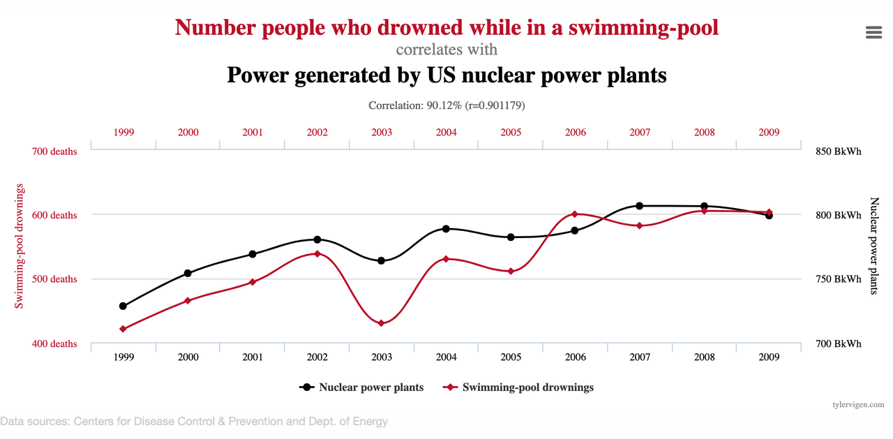
-
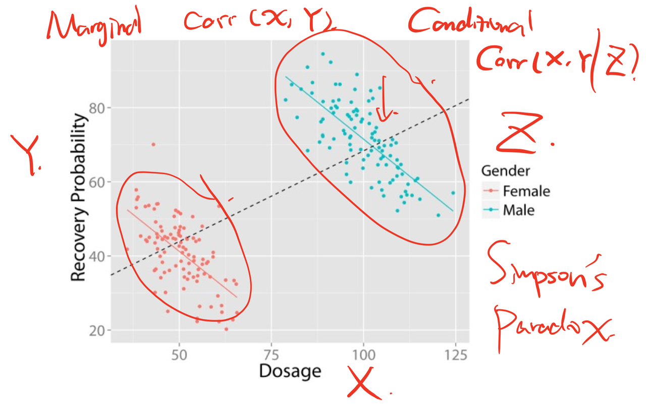
Simpson’s Paradox: The correlation at the subgroup level is inconsistent with the correlation at the overall level.
- For example:
- Gender / Treatment vs Recovery Rate
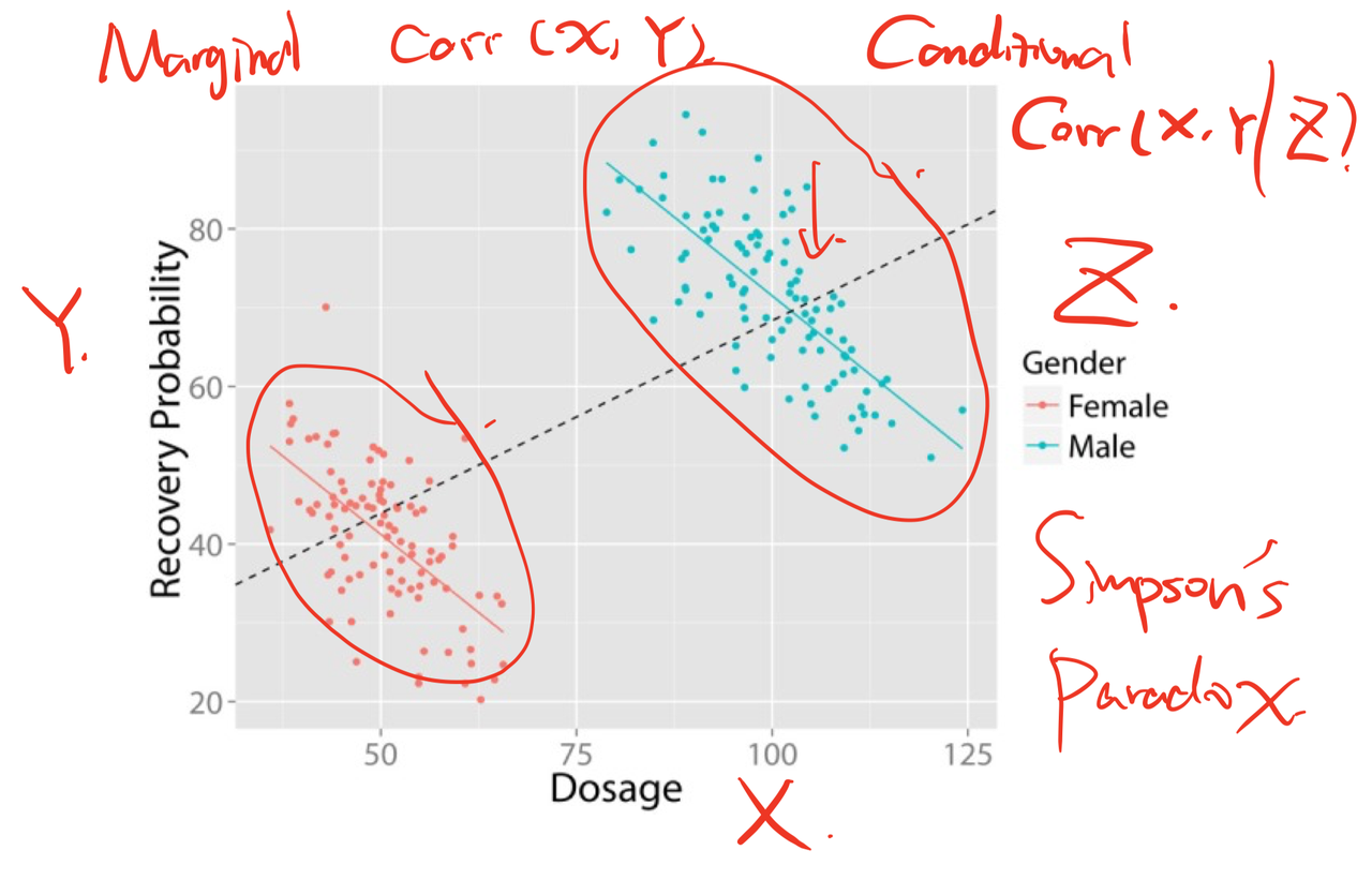
- Similarly: Gender / Watch Time vs Purchase Rate
- Gender / Treatment vs Recovery Rate
- When should we look at subgroup conclusions, and when should we look at overall conclusions?
- Confounding Bias: Correlation caused by a common cause (Fork).
- It affects both the treatment and the effect, but is not affected by either. For example, gender affects whether someone takes medication and also affects the disease rate; but taking medication cannot affect gender.
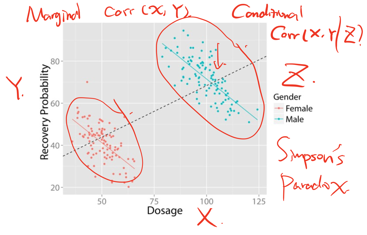
- In this case, we should look at the subgroup data.
- It affects both the treatment and the effect, but is not affected by either. For example, gender affects whether someone takes medication and also affects the disease rate; but taking medication cannot affect gender.
- Selection Bias: Correlation caused by a common effect (Collider).
- It is affected by the treatment and also affects the result (known as a “Mediator”). For example, blood pressure is a mediator through which a drug acts; taking the drug may cause changes in blood pressure, which in turn affects whether one recovers.
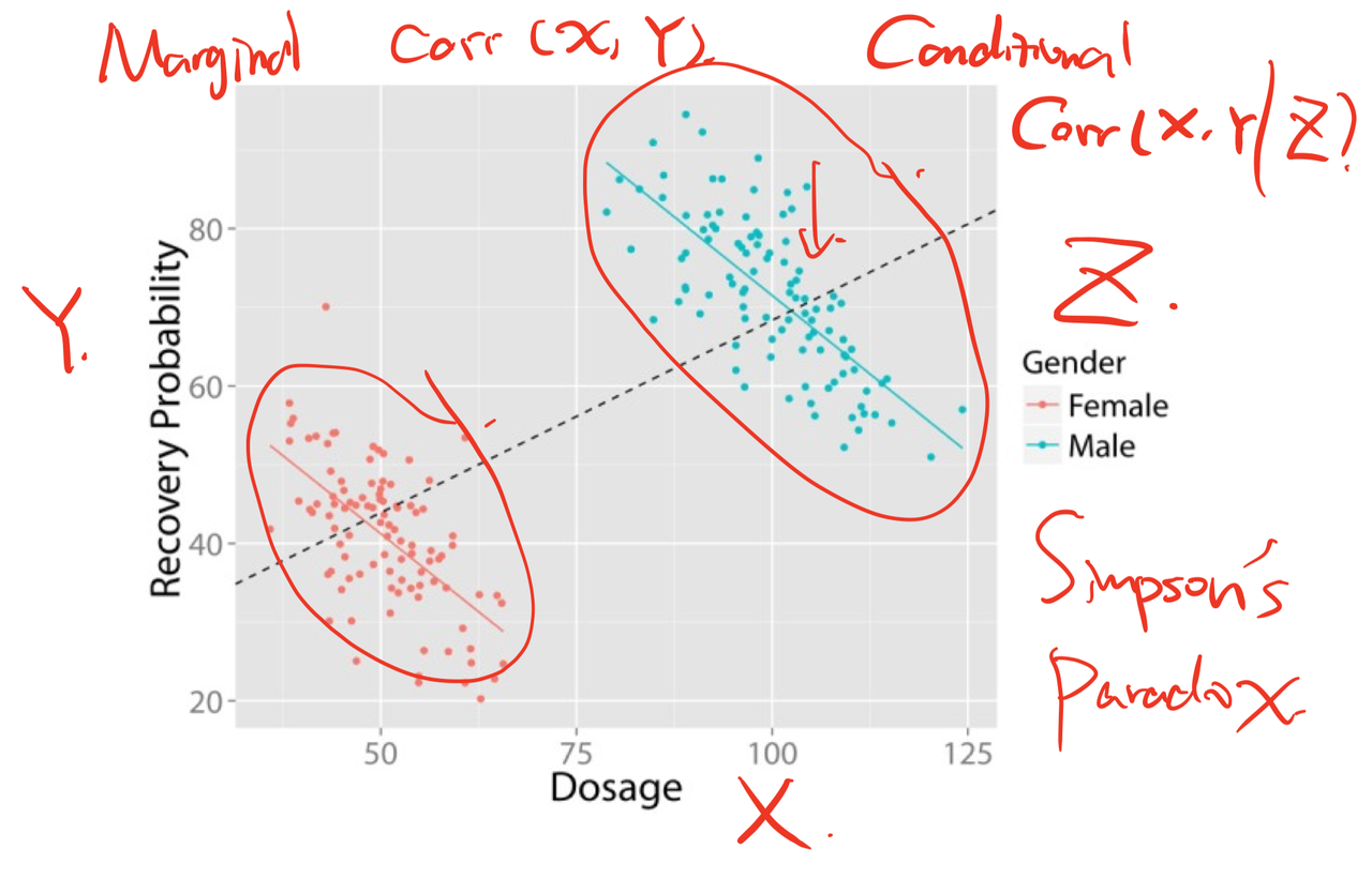
- In this case, to determine the effect of the drug on recovery, we should look at the overall data, rather than dividing the data by blood pressure. Dividing the data here would introduce “selection bias.”
- It is affected by the treatment and also affects the result (known as a “Mediator”). For example, blood pressure is a mediator through which a drug acts; taking the drug may cause changes in blood pressure, which in turn affects whether one recovers.
- Confounding Bias: Correlation caused by a common cause (Fork).
- For example:
-
Berkson’s Paradox: An example of selection bias.
- The better the resume, the worse the ability: candidates who are bad at both will be filtered out, while companies cannot afford candidates who are excellent at both, so they won’t be hired either.
- Similarly, filtering married individuals by IQ and appearance, or “poor families producing noble sons,” are all under the influence of this paradox.
- The better the resume, the worse the ability: candidates who are bad at both will be filtered out, while companies cannot afford candidates who are excellent at both, so they won’t be hired either.
In practical problems, causal relationships may not be so simple and clear:
- For example, the relationship between gender, position, and salary.
- Causal feedback loops: For example:
- Search affects social networking, social networking affects content consumption, content consumption affects search;
- Likes affect traffic, traffic affects GMV, GMV affects traffic, traffic affects likes;
- Mathew Effect: Highly popular content receives further exposure, creating a mutually reinforcing loop.
The Attribution Dilemma: In many models or data analyses, we look backward from the result to find the cause, often optimizing for explanatory power. However, high explanatory power does not mean the attribution is correct.
- For example:
- Explaining sleep quality: Sleeping with shoes on vs. sleeping without shoes on has high explanatory power for sleep quality, but the real cause is that people who get drunk sleep with their shoes on.
- Does providing more content to active community users further increase their community consumption? The causal relationship to be answered here is whether users being more active and liking exploration leads to (causes) consumption.
- For example: it might be that users simply like the app in the first place, which causes them to both consume more and leave more comments in the community. We cannot simply attribute consumption to content and draw a business conclusion.
- Finding the cause backward from the result is a problem with no perfect solution.
- Paper 1: Pearl, J. (2015). Causes of Effects and Effects of Causes. Sociological Methods & Research, 44(1), 149-164. https://doi.org/10.1177/0049124114562614
- Paper 2: Mueller, S., Li, A., & Pearl, J. (2021). Causes of effects: Learning individual responses from population data. https://arxiv.org/pdf/2104.13730.pdf
What: The Counterfactual Problem
Setting aside complex philosophical definitions, let’s focus on the most practical part of the definition of causality (the part that helps your work the most).
- In one sentence: causality attempts to answer “what-if” questions. That is, if everything else remains unchanged, and we only change , does the value of change? If so, we consider that has a causal relationship, or more accurately, causes .
- Let be “whether to undergo surgery” and be “whether the individual survives after one year”. Each individual has two potential outcomes: the outcome after undergoing surgery, and the outcome without undergoing surgery. The difference between these two outcomes is the causal effect of the surgery on survival.
- In reality, we can only observe one potential outcome for an individual. Therefore, individual-level causal effects cannot be determined. This dilemma is called the Fundamental Problem of Causal Inference, which is essentially a missing data problem.
The goals of causal inference methods and models are to solve this counterfactual problem.
How: Experiments & Learning Causal Effects from Observational Data
A/B Testing
Why can randomized A/B testing overcome the missing data barrier? In one sentence: because randomization guarantees that the potential outcomes of both groups are identical in expectation.
- The essence of a randomized trial is that the assignment mechanism (i.e., user assignment) is independent of the potential outcomes. In reality, countless factors affect each person’s potential outcomes, many of which are unobservable. But we no longer need to worry about this, because randomization itself guarantees that user grouping is independent of potential outcomes. In other words, the treatment and control groups are exchangeable, so each group’s potential outcomes can be considered as the overall potential outcomes. Therefore, direct comparison yields the causal effect (assuming a large sample size, ignoring sampling variance).
- This is why internet companies attach great importance to A/B testing. Compared to other methods, A/B testing gives us the opportunity to capture causal effects, thereby helping make business decisions. Although everyone says “data-driven,” having data is not enough to drive decisions! Only data obtained through A/B testing can better drive the business.
Limitations of Experiments:
- When the goal is set, it can tell us which of two paths is better (local optimization), but it cannot tell us where the paths lead.
- Experiments cannot directly answer questions about causal mechanisms: the observed metric difference only shows the effect of the strategy change, not how the effect came about or what the intermediate process was. To understand mediators or mechanisms, we may need to design separate experiments, which can be difficult when the mediators cannot be directly manipulated.
- Effect of cause and cause of effect: Similar to the above, this is not unique to experiments. The estimation methods we introduce all estimate the “effect of a cause,” rather than the “cause of an effect” (the attribution of a phenomenon or result).
Learning Causal Effects from Observational Data
However, in many scenarios, we cannot run experiments. How do we perform causal inference on observational data?
Core: Answer causal questions from observed data through estimation.
- What is estimation: Estimating the estimand using an estimator.
- Estimand: The quantity to be estimated (the question we really want to answer): it is a “what if” question. Due to the counterfactual dilemma, we cannot observe the missing part of the data.
- Estimate: The approximation of the estimand using a finite data sample. It is the actual result obtained, which can only rely on the existing data.
- Estimator: The method or formula used to derive the estimate of the estimand. Its core is to estimate unknown data or parameters.
- How to estimate: Build statistical, machine learning, or various models to remove bias, simulate missing data, or simulate the data generation process to approximate counterfactual questions.
- Whether it can be answered: Identifiability—whether the causal effect can be identified from the data.
- In a general sense, “identifiability” refers to whether a model can yield an output or “has a solution.” For example, in a linear regression model, if there is no data for in all training data, no matter how much data there is, cannot be estimated.
Two Frameworks:
- Rubin Causal Model (RCM) or Potential Outcomes Framework, proposed by Rubin in the 1970s.
- Advantages: RCM defines causal relationships as the comparison between facts and counterfactuals, which is relatively easy to understand and apply. It is suitable for causal inference on observational data and is widely used in social sciences, econometrics, etc.
- Disadvantages: RCM assumes that potential counterfactuals are comparable, meaning the treatment and control groups are similar in other aspects. Its series of assumptions are generally quite strong.
- Structural Causal Model (SCM) or Causal Diagram, proposed by Judea Pearl in the 1980s.
- Advantages: SCM provides intuitive causal diagram representations, helping researchers visualize and understand relationships between variables. It is suitable for complex causal modeling and is widely used in computer science, causal discovery, etc.
- Disadvantages: SCM can be difficult to model for very complex causal relationships, and its causal inference capability on observational data can be limited. Additionally, SCM faces difficulties when dealing with unobserved confounding variables.
| Feature | Rubin Causal Model (RCM) | Structural Causal Model (SCM) |
|---|---|---|
| Proposed Time | 1970s | 1980s |
| Core Concept | Potential outcomes framework, focusing on the comparison of facts and counterfactuals | Causal diagrams, focusing on structural relationships between variables |
| Applicable Fields | Social sciences, econometrics, observational causal inference | Computer science, artificial intelligence, causal discovery |
| Mathematical Basis | Probability theory, statistics | Graph theory, probability theory |
| Main Advantages | 1. Intuitive concept, easy to understand and apply 2. Suitable for processing observational data 3. Closely related to RCT theory 4. Mature estimation methods |
1. Provides intuitive causal diagram representations 2. Suitable for processing complex causal relationships 3. Can handle intervention and counterfactual reasoning 4. Helps understand causal mechanisms |
| Main Limitations | 1. Strong assumptions 2. Difficult to handle complex interactions 3. Sensitive to unobserved confounders 4. Not suitable for dynamic systems |
1. Difficult to model complex systems 2. Limited inference capability on observational data 3. Difficult to handle unobserved confounders 4. High computational complexity |
| Application Scenarios | 1. Policy evaluation 2. Medical research 3. Social science experiments 4. Economic research |
1. Machine learning 2. Artificial intelligence 3. Complex system analysis 4. Causal discovery |
| Tool Support | 1. R packages 2. Stata and other statistical software 3. Traditional statistical methods |
1. Python causal inference libraries 2. Bayesian network tools 3. Graphical model software |