Challenges in A/B Testing
- Challenges in A/B Testing
Overview
| Problem Type | Challenge | Problem Description | Solution | Examples |
|---|---|---|---|---|
| Sensitivity & Statistical Power | Small Treatment Effects | How to deal with small gains when the sample size is insufficient? | Variance Reduction / CUPED | Capping ad value metrics for deep conversion; using CUPED on the ad/campaign side to reduce variance. |
| Triggered Analysis | How to estimate overall platform gains from locally significant gains? | Reverse estimate ATE using ATT and penetration rate. | Combining IV and PSM under experimental scenarios to measure causal effects. | |
| Heterogeneous Treatment Effects | How to identify different individual responses to the same treatment (heterogeneity)? | Linear models / KNN / Causal Forest / Double Machine Learning | User research experiment decompositions (e.g., how client loading strategy variables affect user activity across groups to identify user sensitivity to ads). | |
| Experimental Design & Decision Mechanisms | Long-Term Effects | How to measure long-term changes in short-term experiments to avoid short-sighted decisions? | Predicting long-term outcomes using short-term experiment results | In mid-to-high ad side experiments, estimating learning effects and intermediate metrics to drive and predict long-term LTV trends, where prediction strongly relies on learning effect curves. |
| Optional Stopping | How to avoid cherry-picking results during continuous monitoring? Is simple continuous peek testing NG? | Sequential testing | No actual production application yet; plotting p-value curves over time acts as a surrogate workflow. | |
| Interference | How to handle spillover and mutual interference between units? | Cluster-based experiments / Switchback / TSR method | Budget-based traffic splitting. |
Measurement Problems: Sensitivity and Statistical Power Improvement
Sensitivity Improvement
In the hypothesis testing process of A/B testing, there is an “impossible trinity”: “small effect size, high variance, and small sample size.” In practical applications, such as commercialization scenarios, this challenge is ubiquitous. For example, the sparsity of conversions in deep conversion products leads to high variance in advertiser value. The impact of a single strategy is often in the “basis point” (ten-thousandth) range, usually requiring long observation periods and massive sample sizes to achieve statistically significant results. However, most online traffic experiments are scheduled in weekly cycles and have limited traffic; dealing with small effects and insufficient sample sizes is an inevitable issue, and simply extending experiment duration hurts iteration speed.
How to improve metric sensitivity? Common approaches include:
- Increase Sample Size
- For example, using interleaving experiment mechanisms to replace traditional A/B testing in recommendation/search rankings.
- Improve Sample Quality
- Trimming (Removing outliers): Discarding extremely anomalous observations from the data.
- Removing high-variance/outlier samples.
- Triggered Analysis (detailed below).
- Modify Metric Definitions
- Discretization: Converting continuous metrics into ratio-type metrics by applying thresholds (binarizing count metrics), such as transforming raw impression counts into “proportion of content with impressions > X”, or active days per capita into “active for at least 5 days”. -> A key selection principle for such metrics is ensuring directionality—if the original metric increases in the experiment, the binarized version should also increase.
- Fitting New Metrics: Using machine learning to find the most explanatory variables for the target metric while preserving directionality, and fitting a new proxy metric that has lower variance (Yandex and Facebook have used this approach).
- Variance Reduction
- Capping: Replacing values that exceed a certain threshold (which are logically sound but extreme) with the threshold itself. For example, capping live-stream tips over $500 at $500 to reduce the metric’s variance.
- Assumption: Assumes the treatment only affects uncapped values or affects capped and uncapped values proportionally.
- Challenge: Thresholds are hard to define and may be unstable across different experiments.
- Utilizing Pre-Experiment Data
- CUPED (Controlled Experiments Utilizing Pre-Experiment Data)
- Paper: Deng et al. Improving the Sensitivity of Online Controlled Experiments by Utilizing Pre-Experiment Data.
- Requires strong correlation between pre- and post-experiment metrics (e.g., user active duration).
- Post-Stratification / Variance-Weighted Estimator: Using weighted estimators based on individual-level variance estimates to reduce the variance of the treatment effect estimate. It has been proven that the coefficient of variation of the population variance is a sufficient statistic for determining the scale of achievable variance reduction.
- Optimal Sampling Methods: Using improved sampling methods to improve sensitivity depending on the scenario.
- Karmarkar-Karp heuristic
- Stratified sampling (achieves overall variance reduction when between-strata variance is much smaller than within-strata variance)
- Post-stratification
- CUPED (Controlled Experiments Utilizing Pre-Experiment Data)
- Capping: Replacing values that exceed a certain threshold (which are logically sound but extreme) with the threshold itself. For example, capping live-stream tips over $500 at $500 to reduce the metric’s variance.
- Non-parametric Testing
- For example, Mann-Whitney U test, etc.
CUPED Example:
Let the random variable represent the user’s metric (e.g., app usage duration Stay_Duration) during the experiment phase. represents the average usage duration. Suppose we have another random variable , which in CUPED is typically the user’s pre-experiment metric (e.g., the user’s app usage duration before the experiment started). We define a new adjusted metric:
Y_{adj} = Y - \theta X + E(\theta X)$$ (Formula 1) where $E(X)$ is the theoretical expectation of $X$, which is a constant parameter. At this point: $$E(Y_{adj}) = E(Y - \theta X + E(\theta X)) = E(Y) - \theta E(X) + \theta E(X) = E(Y)
This means is an unbiased estimator of .
Meanwhile:
= \frac{1}{n}(Var(Y) + \theta^2 Var(X) - 2\theta Cov(Y,X))$$ (Formula 2) Note that the variance of the new metric is a quadratic function of $\theta$, representing an upward-opening parabola. When: $$\theta = \frac{Cov(Y,X)}{Var(X)}
achieves its minimum value.
Triggered Analysis
- Certain strategies require active user behaviors to “opt-in,” such as signing up to receive a reward, or taking specific actions to trigger the treatment. This creates a funnel where the Average Treatment Effect (ATE) is diluted by the “penetration/trigger rate.”
- Triggered Analysis improves sensitivity by analyzing only the users who were actually triggered by the strategy (e.g., users who entered the payment page). Although this reduces the sample size, it prevents the treatment effect from being diluted by non-triggered users. If the proportion of triggered users is very small, ATE will be significantly underestimated. In this case, looking only at triggered users is a great way to mitigate dilution. The two main challenges are:
- Extrapolating results from triggered users to the overall population.
- Reducing the variance of the ATE estimate to offset the sensitivity loss caused by the smaller sample size of triggered users.
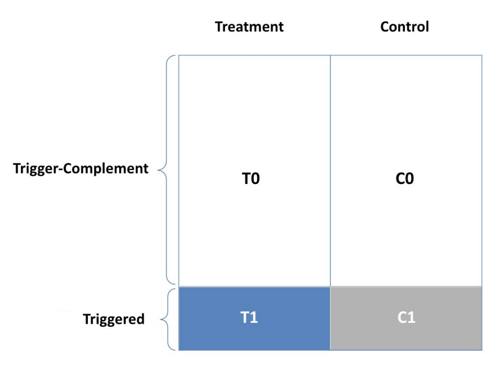
- Method 1: User-Triggered Analysis (Commonly used)
- Sample selection: Observe triggered users from their first trigger event, analyzing all events during the experiment cycle.
- Advantages: No assumptions are made about the treatment effect; allows looking at user-level metrics. It has been proven to improve statistical power and reduce variance.
- Method 2: Session-Triggered Analysis
- Sample selection: Observe triggered users only during the sessions in which they were triggered.
- Pros/Cons: Stronger variance reduction than user-triggered analysis, but relies on a strong assumption: the treatment effect only occurs within the triggered session.
- Estimation: Diluted Formulas
- Example:
-
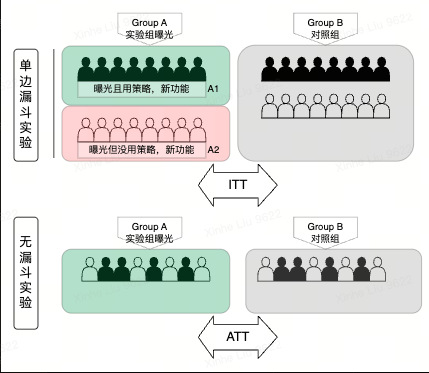
- ITT (Intention-to-treat): Measures the average effect on the intended population (the entire treatment group ), which includes users who did not actually adopt the strategy.
- ATT (Average treatment effect on the treated): Measures the average effect on the actual adopters of the strategy.
-
- Find comparable groups and , and use ATT to back-calculate ATE/ITT:
- Absolute effect:
- Ratio metrics: , where is the average trigger rate (the function of the denominator).
- Can be combined with methods like CUPED to reduce variance.
- Example:
- Common Questions
-
Can the idea of using Instrumental Variables (IV) to estimate ATT be applied to scenarios with “always-takers”?
-
The estimators are not exactly the same. IV estimates the Local Average Treatment Effect (LATE), which is the treatment effect on the compliers. In the absence of always-takers, the estimate for is equivalent to the estimate for compliers, meaning LATE = ATT. However, when always-takers exist, the compliers estimated by IV are only a subset of the treated units, which does not represent the ATT of all adopters. Thus, estimating via 2SLS (Two-Stage Least Squares) and PSM (Propensity Score Matching) will yield different estimators.
T = 0 T = 1 Z = 0 Never-taker + Complier Always-taker Z = 1 Never-taker Always-taker + Complier
-
-
Can the ATT estimate be extrapolated to the entire population? For example, if a feature has a significant effect on compliers, can we roll out the feature to everyone (e.g., from manual click to pop-up window) and assume the effect will be equal to the estimated ATT?
- No. Compliers are self-selected, and their distribution differs from the overall population. The ATT estimated on compliers does not represent the effect on the general population. If a significant conclusion is observed on compliers and you consider changing the product logic (such as making a manual opt-in automatic), you must run a new experiment to measure the actual effect on the overall population.
-
How to find a comparable sample in the control group for ?
- Using Instrumental Variables (IV)
- The random assignment in A/B testing itself is a perfect instrumental variable. We only need to know the proportion of compliers in the treatment group to estimate the causal effect.
- Assumptions:
- : The effect of on is mediated entirely through ; no backdoor paths exist between and ; monotonicity assumption (), meaning there are no defiers or always-takers, only compliers and never-takers.
- Challenge:
- IV itself does not improve sensitivity or significance. In scenarios with a funnel, if the ITT (reduced-form estimation) from A/B testing is not significant, the LATE estimated by the instrumental variable is highly unlikely to be significant either.
- The significance of IV estimation is basically identical to that of the reduced-form estimation. Thus, LATE is not a tool for increasing statistical significance. The motivation for using LATE is usually driven by the business question—we care about the effect of adopting the strategy, not the effect of the nudge from random assignment.
- Assumptions:
- The random assignment in A/B testing itself is a perfect instrumental variable. We only need to know the proportion of compliers in the treatment group to estimate the causal effect.
- For the same endogenous variable/strategy, using different instrumental variables will yield different LATEs. This is because different IVs affect different sets of compliers, acting on different subgroups, which naturally leads to different treatment effects.
- Counterfactual Logging
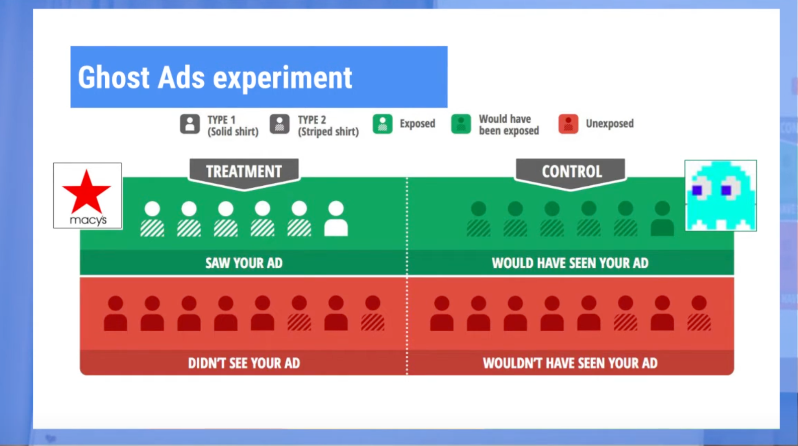
- Identifying a comparable group in the control group through system logging (e.g., having the model predict twice).
- This can significantly reduce variance to estimate ATT.
- However, the engineering cost is very high.
- Example: The “Ghost Ads” mechanism used in advertising scenarios (Reference: Johnson, G. A., Lewis, R. A., & Nubbemeyer, E. I. (2017). Ghost Ads: Improving the Economics of Measuring Online Ad Effectiveness., YouTube).
-
- Limitations:
- Ghost ad thresholds: Raises questions about whether a single ghost ad trigger is an accidental recommendation event and how many triggers are needed to be truly comparable.
- Strategy interference: Once a ghost ad is triggered, frequency capping and other ad pacing rules might cause the control group’s trigger probability to rise. Therefore, the experiment cannot run for too long.
- Example: The “Ghost Ads” mechanism used in advertising scenarios (Reference: Johnson, G. A., Lewis, R. A., & Nubbemeyer, E. I. (2017). Ghost Ads: Improving the Economics of Measuring Online Ad Effectiveness., YouTube).
- Matching Methods
- Finding a comparable control group using pre-experiment features (e.g., Propensity Score Matching - PSM).
- The estimation might have bias, but it improves sensitivity.
- Often used in tandem with IV (Two-stage estimation).
How to combine IV and Propensity Score Matching (PSM)?
IV Calibration"] H --> I{"Significant?
& Passes IV Test"} I -- Yes --> J["Output ATT"] I -- No --> K["No significant effect
Optimize strategy & restart experiment"] style D fill:#d4efdf,stroke:#2ecc71 style G fill:#d4efdf,stroke:#2ecc71 style J fill:#d4efdf,stroke:#2ecc71 style K fill:#fadbd8,stroke:#e74c3c style A fill:#fadbd8,stroke:#e74c3c
How to combine matching methods to reduce bias? Taking Two-Stage Regression as an example:
Assume a linear relationship between strategy and outcome : .
Under this assumption, the treatment effect ATT = is the same for everyone. We can derive that using an IV can yield an unbiased estimate of the ATT under IV assumptions A1 - A4:
Variable Type - Unbiased Estimation Inference
When Y and T are both binary (0, 1) variables:
\begin{align*} \delta&=\frac{E[Y|Z = 1]-E[Y|Z = 0]}{E[T|Z = 1]-E[T|Z = 0]}\\ E[Y|Z = 1]-E[Y|Z = 0]&=E[\delta T+\alpha _u U|Z = 1]-E[\delta T+\alpha _u U|Z = 0] \ ( \text{Assumption 2 and 4} )\\ &=\delta (E[T|Z = 1]-E[T|Z = 0])+\alpha _u (E[U|Z = 1]-E[U|Z = 0])\\ &=\delta (E[T|Z = 1]-E[T|Z = 0])+\alpha _u (E[U]-E[U]) \ ( \text{Assumption 3} )\\ &=\delta (E[T|Z = 1]-E[T|Z = 0])\\ \delta&=\frac{E[Y|Z = 1]-E[Y|Z = 0]}{E[T|Z = 1]-E[T|Z = 0]} \end{align*}
IV Assumption 1 ensures the denominator . is the ATT we want to estimate. The conditional expectations in the numerator and denominator can be calculated from the conditional averages in the experimental data.
If there are no always-takers in the experiment, there are no users in the control group. represents the penetration rate in the treatment group, in which case ATT equals ITT / penetration rate.
When Y and T are continuous variables:
\begin{align*} \delta&=\frac{Cov(Y,Z)}{Cov(T,Z)}\\ Cov(Y,Z)&=E[YZ]-E[Y]E[Z]\\ &=E[(\delta T+\alpha _u U)Z]-E[\delta T+\alpha _u U]E[Z] \ ( \text{Assumption 2 and 4} )\\ &=\delta (E[TZ]-E[T]E[Z])+\alpha _u (E[UZ]-E[U]E[Z])\\ &=\delta Cov(T,Z)+\alpha _u Cov(U,Z)\\ &=\delta Cov(T,Z) \ ( \text{Assumption 3} )\\ \delta&=\frac{Cov(Y,Z)}{Cov(T,Z)} \end{align*}
Assumption 1 ensures the denominator .
Two-Stage Least Squares (2SLS): Applicable to all variable types
- , yielding predicted values . First stage: Regress on .
- . Second stage: Regress on . At this point, is mapped from through the first-stage regression, inheriting ’s unconfoundedness.
Adding covariates that are highly correlated with and in the two-stage regression can reduce the estimation variance (similar to the CUPED approach).
The advantage of linear models is that they can utilize IV to calculate an unbiased ATT estimate of on . However, their limitation is also obvious: the linear model assumes that the treatment effect is the same for everyone.
Heterogeneous Treatment Effect (HTE)
Sometimes, focusing only on the overall treatment effect (ATE) does not meet our needs. For example:
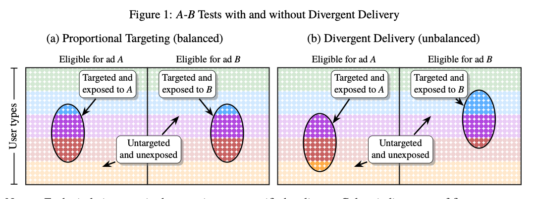
- In an ad strategy experiment, due to user self-selection or recommendation strategies, there are differences in the target populations reached.
- From the overall strategy effect, treatment is superior to . However, in head-to-head subgroup comparisons, ’s content quality/conversion rate is superior to ’s.
-
Experimental Mechanisms and Decision-Making Problems
Long-Term Effects
Due to cost and iteration speed constraints, standard experiments evaluate the short-term effects of a strategy. However, businesses ultimately care about long-term effects. We usually assume that short-term effects represent long-term effects, but this does not always hold true.
Reasons why short-term effects may fail to represent long-term effects include:
- User learning over time causes the treatment effect to change (i.e., ATE is a function of time).
- Novelty Effect: A fresh change initially captures user attention and drives engagement, but this effect fades or even reverses over time.
- Poor search results cause users to search repeatedly. In the short term, search queries and ad revenue rise; in the long term, users leave, and revenue falls.
- Showing more ads increases short-term revenue, but users may churn or learn to ignore ads, causing long-term revenue to decline.
- Primacy Effect: A change might not show positive gains initially, but as users adapt to the change, engagement increases over time.
- Novelty Effect: A fresh change initially captures user attention and drives engagement, but this effect fades or even reverses over time.
- The strategy effect itself takes time to manifest.
- Delayed Network Effects: Network effects in social or platform products take time to accumulate; short-term experiments cannot observe the value brought by reaching critical mass.
- Habit Formation Cycle: Forming new habits takes weeks or even months; short-term experiments struggle to capture the establishment of stable behavior patterns.
- On Airbnb, the time from booking to check-in is long; the impact on user retention takes a long time to measure.
- Long-Tail Effects: Certain strategies may impact a minority of users significantly, but it takes time for this to manifest in overall metrics.
- Cross-Platform Synergy: User behavior migration and adaptation across multiple platforms take time to evaluate fully.
- Brand Perception Building: Certain changes may affect brand perception, an effect that takes a long time to manifest in user behavior.
- Ecosystem/External Shifts: New feature rollouts, seasonality, competitive landscape changes (e.g., competitors launching the same feature), regulatory changes (e.g., GDPR), concept drift, and software degradation can all cause strategy effects to decay.
Method 1: Long-Term Experiments
The most intuitive method is to extend the experiment duration. The following analysis methods are typically used:
- Direct Analysis
-
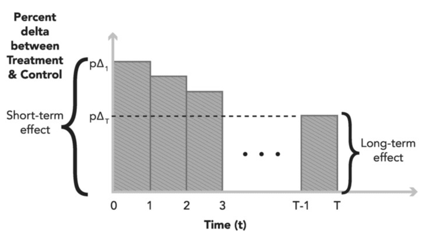
- For attribution: Effect Dilution
- Effect dilution caused by users using multiple devices.
- If assignment is based on cookies, the longer the duration, the more likely a natural person enters both the treatment and control groups.
- If network effects exist, the longer the duration, the greater the leakage.
- Survivor Bias: If user retention differs between groups, looking only at the last week of data does not accurately reflect the treatment effect.
- Interaction with other features: Many new features are launched during the experiment, which affects the performance of existing features. For example, sending pushes might be highly effective initially, but if other teams also start sending pushes, the effect will decay.
- If the external environment changes, the experimental effect will also be affected, so the difference between the end and start of the experiment is not necessarily due to the strategy itself.
-
- Cohort Analysis
- Analyzing the short-term and long-term effects of the same cohort of users can solve dilution and survivor bias, but two questions must be considered:
- First, confirm the stability of the user identifier. The identifier (e.g., UID) must remain stable across the experiment cycle.
- Does this cohort represent the overall user base? If not, the external validity of the experiment will be very low (e.g., for low-frequency businesses, users who enter the experiment early might be highly active power users).
- Analyzing the short-term and long-term effects of the same cohort of users can solve dilution and survivor bias, but two questions must be considered:
- Post-Period Analysis
-
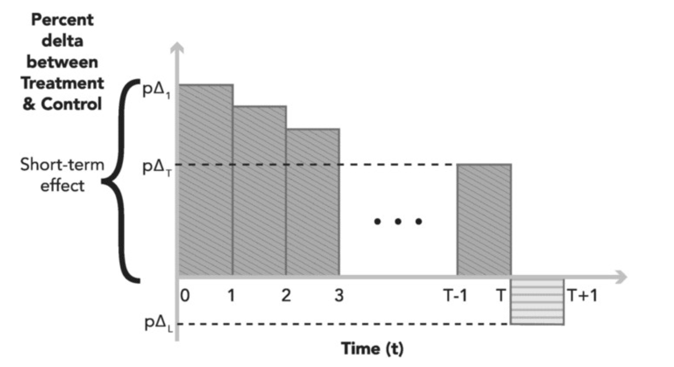
- Comparing treatment and control users after the experiment is turned off to measure user learning. During this phase, both groups receive the same treatment, so the measured difference represents the learning effect, which can be categorized into:
- User learning effect: For example, after showing users many low-quality ads, users learn to click ads less frequently.
- System learning effect: The system “remembers” prior information, particularly for machine learning models (e.g., algorithms that show more ads to users who tend to click ads. If the experiment caused users to click more ads, they will continue to see more ads even after the experiment ends).
-
- Time-Staggered Treatments
- Both groups receive the same treatment, but start at different times. The effect is measured by comparing the two groups.
-
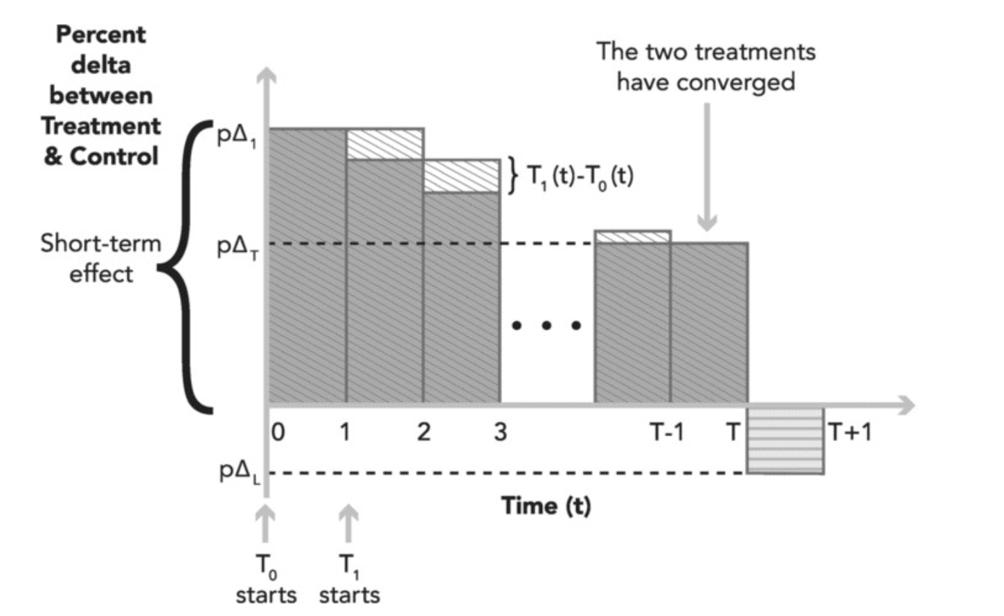
- Holdback and Reverse Experiment
- High experimental cost.
- The experiment runs for too long to make agile decisions.
- Cannot control other variables over a long period.
- For example, users cannot be tracked continuously, or a single device is shared by different users.
- Or a user logs in using different devices over time, which pollutes the assignment.
Long-term experiments face several challenges compared to short-term experiments:
- Cookie Stability Issues
- Cookie Churn: Low cookie retention (less than 25% over two months) leads to sample loss and selection bias.
- Avoidance: Use UID/Device ID for assignment or implement cookie backup mechanisms.
- Cookie Clobbering: Data loss due to non-user-initiated clears (e.g., browser bugs).
- Avoidance: Conduct cross-browser compatibility testing and set up redundant data storage.
- Cookie Churn: Low cookie retention (less than 25% over two months) leads to sample loss and selection bias.
- Experimental Design Bias
- Survivor Bias: User churn makes the remaining sample unrepresentative (e.g., highly active users are more likely to remain).
- Avoidance: Use churn-resistant metrics (e.g., Click/User) and track users across the full lifecycle.
- Selection Bias: PP (Post-Period) methods might overestimate learning effects (e.g., ad underline experiments).
- Avoidance: Verify short-term conclusions by comparing them with direct observations from long-term experiments.
- Survivor Bias: User churn makes the remaining sample unrepresentative (e.g., highly active users are more likely to remain).
- Effect Confounding
- Mixing of short-term and long-term effects: User learning (ad adaptation) is interwoven with system-level or seasonal changes.
- Avoidance: Use the CCD method (detailed below) to quantify learning effect trends.
- Residual side effects: The experiment might still affect user data entry or model feedback loops after it has ended.
- Avoidance: Design strategy rollback monitoring periods and causal impact chains.
- Mixing of short-term and long-term effects: User learning (ad adaptation) is interwoven with system-level or seasonal changes.
- External Interference
- Seasonality: Major events can interfere with learning effect measurements (e.g., entertainment experiments during Grammy week).
- Avoidance: Analyze the full cohort rather than dividing observations into segments.
- Spurious attribution: System-level changes might be misclassified as learning effects (e.g., shifts in browser market share).
- Avoidance: Establish system change baselines and implement multi-dimensional attribution models.
- Seasonality: Major events can interfere with learning effect measurements (e.g., entertainment experiments during Grammy week).
- Methodological Limitations
- Naive Setup: Vulnerable to system, seasonal, or interaction interference. (Optimization: Combine with counterfactual prediction models).
- PP Method: Prone to sample churn and selection bias. (Optimization: Shorten the post-period observation window).
- CCD Method: High engineering complexity and requires larger traffic allocation. (Optimization: Deploy phased traffic scaling strategies).
- Metric Design Pitfalls
- Misleading ratio metrics: Metrics like CTR can mask user churn.
- Avoidance: Monitor absolute count metrics (e.g., total clicks) alongside ratio metrics.
- Incomplete convergence: The learning effect might not fully converge within the experiment cycle.
- Avoidance: Use exponential decay models to extrapolate effects.
- Misleading ratio metrics: Metrics like CTR can mask user churn.
- Key Validation Steps
- Conduct A/A tests before the experiment to verify balanced traffic split.
- Periodically check user profile consistency between groups.
- Build counterfactual control groups to exclude external interference.
- Perform sensitivity analysis and cross-method validation on significant findings.
Method 2: Modeling User Learning
- Google proposed a new experimental mechanism:
- Reference: Hohnhold, H., O’Brien, D., & Tang, D. (2015). Focusing on the Long-term: It’s Good for Users and Business. KDD (pp. 1849-1858).
- This solves the problem of long-term effects being hard to measure (fitting learning effects with parameters) and noise issues (long experiment duration allows external interference to mix in).
- Cookie-Cookie-Day (CCD) Experimental Mechanism
-
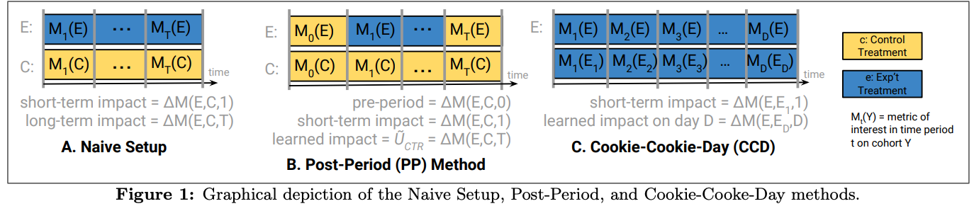
- The CCD framework combines two parallel experiments:
- Standard Cookie Experiment: Users remain in fixed treatment or control groups throughout.
- Cookie x Day Experiment: Users are randomly reassigned to treatment or control groups every day. This dual approach isolates long-term effects by comparing cohorts with continuous exposure to those with transient exposure. The daily rerandomization in the Cookie x Day experiment creates a control group experiencing a baseline treatment, enabling researchers to distinguish immediate effects from cumulative learning.
- Challenges:
- When using models to fit residual effects of longer stages, the assumption of might be unreasonable. This paper assumes a learning effect parameter of 0.012, but because the intensity of exposure affects the speed of user learning (e.g., users who search more frequently or see ads more often learn faster), a long experiment duration might not be necessary.
- Using cookies as user identifiers introduces bias; users switch devices, use different browsers, and privacy-conscious users clear cookies regularly.
- If control conditions are not strict, various biases (such as word-of-mouth or user sharing) can slip in.
-
Method 3: Surrogate Index (Short-term Proxies for Long-term Outcomes)
Identify short-term “driver metrics” that have a causal impact on the long-term treatment effect, measure them, and estimate user learning to predict the long-term effect.
Paper 1: Athey, S., Chetty, R., Imbens, G. W., & Kang, H. (2019). The surrogate index: Combining short-term proxies to estimate long-term treatment effects more rapidly and precisely (No. w26463). National Bureau of Economic Research.
- Formalized how to combine intermediate outcomes to estimate long-term effects efficiently, clarified the assumptions under which this method yields unbiased estimates, and formally incorporated the estimation of the relationship between short-term surrogates and long-term outcomes using secondary datasets.
- Developed bounds for the bias that occurs when these assumptions are violated, and out-of-sample methods to validate the assumptions.
- Demonstrated that using surrogates improves efficiency even when long-term effects can be estimated directly.
- Provided an empirical application showing that combining multiple intermediate outcomes (rather than a single predictor) can predict long-term labor market treatment effects years in advance with significantly improved precision.
- Key Takeaways:
- Comprehensive theoretical framework and mathematical proof.
- Practical execution: How to identify surrogates from observational data and validate them using experimental (or quasi-experimental) data.
- Methods to falsify surrogacy/mediation: Hold-out methods.
Paper 2: Yang, J., Eckles, D., Dhillon, P., & Aral, S. (2023). Targeting for long-term outcomes. Management Science. (HBS)
- Main Contributions: An extension of Paper 1.
- Analytically demonstrated under what conditions the surrogate index can effectively replace unobservable long-term outcomes for policy evaluation and optimization.
- Empirically validated the method:
- Conducted two large-scale experiments to determine which incentives to offer which users to maximize long-term subscription revenue for The Boston Globe.
- Combined data from the first experiment with time progression, proving that policies optimized based on the surrogate index outperformed those optimized based on short-term proxies, and performed similarly to policies optimized on actual long-term outcomes.
- Implemented the optimized policy and added extra random exploration to handle potential non-stationarity, updating the policy after each experiment.
- Key Takeaways:
- The theoretical assumptions required for the Surrogate Index framework:
-
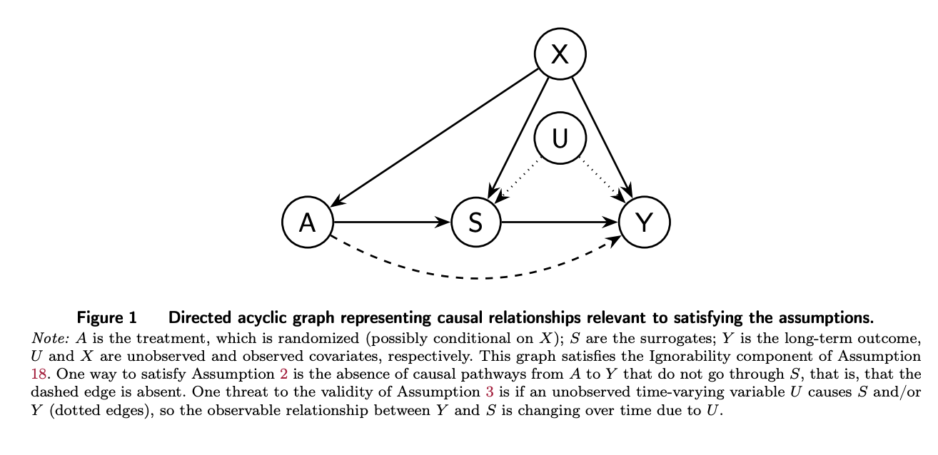
- Unconfoundedness (equivalent to Ignorability, Positivity): Standard causal inference assumptions.
- Surrogacy Condition (Complete Mediation): Can only be falsified; Paper 1 proposes a method.
- Comparability: The distribution of long-term outcomes conditional on covariates and surrogates is the same in the experimental and historical datasets.
In practice, the distribution must not shift between model training and rule formulation.
-
- Practical steps (combining Paper 1 and Paper 2).
- The theoretical assumptions required for the Surrogate Index framework:
Paper 3: Wang, Y., Sharma, M., Xu, C., Badam, S., Sun, Q., Richardson, L., … & Chen, M. (2022, August). Surrogate for long-term user experience in recommender systems (pp. 4100-4109), Google Research.
- Studied a series of continuous user behavior patterns and standardized a workflow to pinpoint subsets of behaviors that have strong predictive power for long-term user revisit frequency.
- Measurement: Proposed metrics to capture sequential and temporal user consumption patterns.
- Insights: Identified user behavior patterns correlated with long-term user experience.
- Surrogate Selection: Standardized the selection of user behavior patterns as surrogates for long-term user experience based on robust predictive models.
- Algorithmic Improvement: Validated the effectiveness of optimizing long-term user experience using surrogates in a reinforcement learning recommendation system.
- The main challenge lies in capturing users’ true interests rather than merely inferring them from topics they previously consumed.
- This requires defining a metric to capture true user interests to improve long-term user experience in recommendation systems.
- Key Takeaways:
- Proxy metrics: definition of diversity, active/high-value consumption (setting thresholds for establishing “mindshare”), category discoverability, and revisit/repurchase frequency.
- Pre-experiment data analysis: verifying path consistency.
- Metric selection: using tree-based methods.
- Validation: reward experiments (running long-term experiments with EE/RF).
Paper 4: Duan, W., Ba, S., & Zhang, C. (2021, March). Online Experimentation with Surrogate Metrics: Guidelines and a Case Study. LinkedIn.
- Key Takeaways:
- The “Surrogate Metrics” in this paper differ slightly from the “Surrogate Index” in the previous three papers, aligning closer to validating the feasibility of using predicted values (e.g., predicted LTV) in place of posterior values in experiments. It is highly practical.
- Practical Principles:
- Guidelines for choosing north star metrics (qualitative rules):
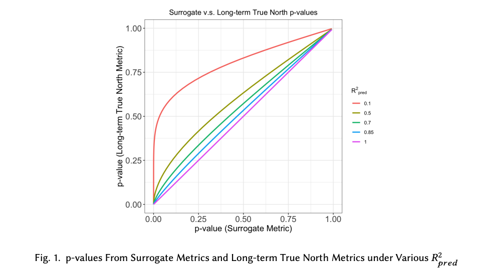
- High predictive power for the true north star metric (high , AUC, etc.).
- Focus on metrics we can change and measure in the short term (analyzing historical experiment leverage).
- Tailor metrics to different treatment characteristics (consistent metric definitions across channels, users, etc.).
- Interpretability (if using a model, fluctuations in the surrogate should be explainable).
- Low administrative overhead (prefer simple rules over models that require continuous training and are hard to explain).
- Experiment variance must be corrected: The variance of surrogate metrics is typically smaller than the actual outcome; the variance of the prediction step itself must be accounted for.
-
- How to validate the surrogacy condition:
- Verify that is the sole path (complete mediation), equivalent to (note that the authors did not control for other variables, assuming all information is captured in the model).
- In real-world applications, use historical experimental data to ensure the deviation is not too large.
- Guidelines for choosing north star metrics (qualitative rules):
Other Methods
Statistical solutions:
- Treating the long-term treatment effect as a bias introduced by heterogeneous treatment effects, and deriving a bias-adjusted jackknife estimator of the ATE based on HTE for specific groups.
- References:
- Günter J. Hitsch and Sanjog Misra. Heterogeneous treatment effects and optimal targeting policy evaluation. Working paper, 2018.
- Eva Ascarza. Retention futility: Targeting high-risk customers might be ineffective. Journal of Marketing Research, 55(1):80–98, 2018.
- References:
- In double-sided market scenarios, using sequential testing and reinforcement learning to validate long-term treatment effects.
- Causal inference:
- Marshall M. Joffe and Tom Greene. 2009. Related causal frameworks for surrogate outcomes. Biometrics 65, 2 (2009), 530–538.
- Ross L. Prentice. 1989. Surrogate endpoints in clinical trials: definition and operational criteria. Statistics in medicine 8, 4 (1989), 431–440.
- Christopher J. Weir and Rosalind J. Walley. 2006. Statistical evaluation of biomarkers as surrogate endpoints: a literature review. Statistics in medicine 25, 2 (2006), 183–203.
- Recommendation systems:
- Wang-Cheng Kang and Julian McAuley. 2018. Self-attentive sequential recommendation. In ICDM’18. IEEE, 197–206.
- Raghav Pavan Karumur, Tien T. Nguyen, and Joseph A. Konstan. 2018. Personality, user preferences and behavior in recommender systems. Information Systems Frontiers 20, 6 (2018), 1241–1265.
Reference: Lassen, et al., 2022. Statistical Challenges in Online Controlled Experiments: A Review of A/B Testing Methodology.
Optional Stopping (Continuous Testing Problem)
The continuous testing problem focuses on how to terminate experiments early without compromising statistical validity. Businesses want to rapidly filter out strategies with positive effects while abandoning negative strategies as early as possible. Because experiment results can be observed in near real-time, researchers are prone to “peeking” behaviors—continually monitoring p-values and stopping the experiment the moment significance is reached. While this reduces experimental costs, it significantly inflates the false positive rate (Type I error). Therefore, we need an early termination mechanism that controls the Type I error rate while allowing early decisions.
Peeking Problem: Continuous monitoring inflates the Type I error rate. If you perform a hypothesis test daily with a 5% significance level, the overall false positive rate over days escalates to .
Sequential Testing
- By lowering the significance level (alpha) of each daily/individual hypothesis test, we ensure that the overall Type I error rate across multiple tests does not exceed 5%.
- Advantages: Controls the Type I error rate, preventing the inflation of false positives caused by stopping experiments the moment they happen to look significant.
- Disadvantages:
- Inapplicable scenarios (e.g., testing multiple metrics simultaneously, which reduces HTE power).
- Sequential testing reduces statistical power. According to Optimizely’s data, this method leads to roughly a 36% loss in statistical power.
- To address the power loss of sequential testing, we split the experiment into two phases:
- Monitoring Phase: From the start of the experiment to the day before it ends, we use a conservative sequential testing method for continuous monitoring. Decisions are made early only if the effect is exceptionally significant and satisfies a minimum observation window, focusing on Type I error control.
- Decision Phase: Once the experiment ends, we use traditional fixed-sample testing for comprehensive analysis and decision-making, focusing on statistical power. This approach controls Type I errors throughout the monitoring phase while maintaining high statistical power in the final decision phase, balancing safety and sensitivity.
- This method requires prior knowledge of the underlying causal distribution, which limits its practical application.
- In Optimizely’s paper, the prior distribution is assumed to be a normal distribution with a mean of 0 and an unknown variance, which can be estimated using the true treatment effect from historical experiments. This aligns with probability-based estimation and fits perfectly with sequential testing.
- Another method converts this into an optimization problem. For Type I error control, we find no restrictions on the prior distribution of parameters. Whether we use a normal distribution with arbitrary variance, a uniform distribution, or a lognormal distribution, we can control the Type I error rate effectively using martingale properties.
Specific Methods:
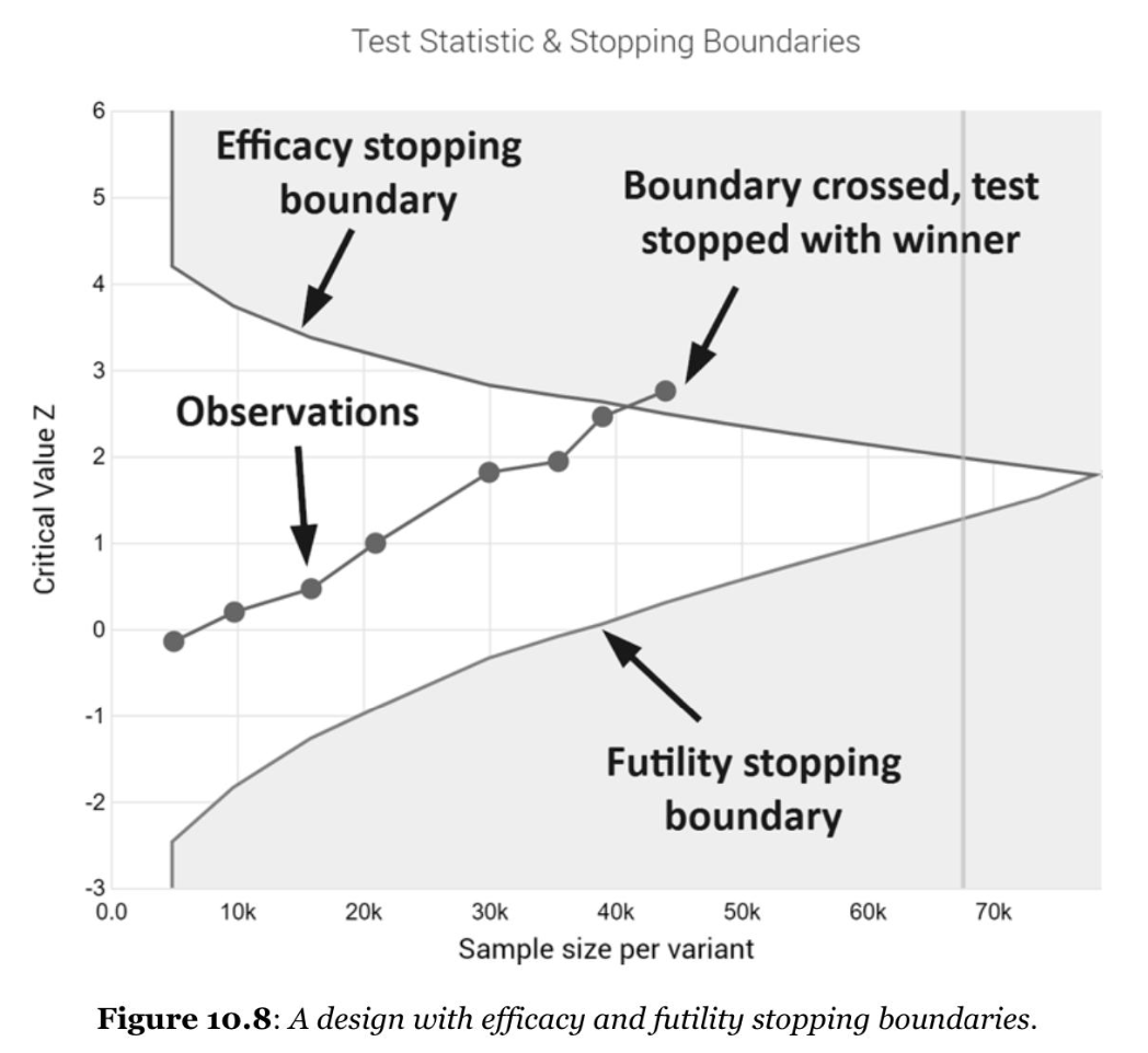
- Sequential Probability Ratio Test (SPRT)
- ; Hypotheses are defined as: .
- Likelihood ratio test statistic: .
- Using boundaries and , the rejection region divides the sample space into three decision rules:
- If , reject and stop the experiment.
- If , fail to reject and stop the experiment.
- If , accumulate more samples and compute .
- Statistical Principles:
- When holds, the likelihood ratio (LR) statistic is a martingale, fluctuating randomly around 1. Thus, we can control the Type I error rate using martingale properties. Using as the threshold to judge LR significance, LR > indicates a significant result. Assuming significance is first reached at test , the Type I error rate over arbitrary multiple tests will not exceed . When we use as the monitoring threshold, the Type I error rate is controlled within , meaning that under , there is only a 5% chance of a false alarm even if we wait indefinitely.
- An awkward problem arises: we do not know if the strategy actually has an effect. When holds, there is a 95% probability that we will never achieve significance. To address this, we use truncation—setting a maximum cutoff time. If no significant conclusion is reached by this cutoff, we assume the strategy has no effect and stop the experiment.
- In the chart, the upper boundary “reject null if crossed” is the Efficacy Boundary. Once crossed, the experiment stops. The lower boundary “accept null if crossed” is the Futility Boundary, used to terminate experiments early to avoid wasting resources.
- Building on this, research has yielded mixture sequential probability ratio test (mSPRT) and generalized sequential probability ratio test (GSPRT).
- Group Sequential Trials (GST): In practice, it is rarely feasible to perform continuous testing (running a test for every single new data point) due to high costs. In GST, the data is divided into several chunks (groups), and tests are run at each stage before combining the results.
- Choosing Decision Boundaries: The more samples accumulated, the more aggressive the boundary.
- Requirement: Analysis intervals must be pre-planned. For example, if conducting two analyses, the first and second must use 50% and 100% of the total information volume. If conducting four analyses, they must use 25%, 50%, 75%, and 100%. The number and timing of analyses must be determined beforehand.
- Improvements: Spending functions (common in clinical trials).
- Group Sequential Trials (GST): In practice, it is rarely feasible to perform continuous testing (running a test for every single new data point) due to high costs. In GST, the data is divided into several chunks (groups), and tests are run at each stage before combining the results.
Sequential testing is widely used in the industry (Netflix uses Group Sequential, Optimizely, Ant Group, and the user-side of Libra). Besides sequential testing, the industry and academia use other methods to address peeking:
| Name | Theoretical Concept | Practical Scenario | Advantages | Disadvantages |
|---|---|---|---|---|
| p-value Curve (Libra’s current scheme) | When continuously checking report significance over multiple days, “considering significance over multiple consecutive days before making a decision” lowers Type I errors compared to “making a decision the moment significance is reached on any single day.” Adjusting the decision logic can control Type I errors within the target alpha. | Making decisions only when “the p-value curve remains stable and significant” prevents Type I error inflation. Optimal decision logic: Day 1 < , Day 2 and 3 < . | 1. Easy to implement in engineering. 2. Type I error control might be slightly loose, and errors may still slightly exceed the target alpha. |
1. High user cognitive and training overhead. |
| mSPRT (Netflix) | Within each sample group, assume all samples are independent and identically distributed (i.i.d.). Reconstruct the p-value calculation so that the observed p-value is always controlled within the target alpha, regardless of when it is checked. This is proved using martingale properties. | In online A/B testing, user revisits break the i.i.d. assumption. Reconstructed p-values lose their martingale properties, introducing a risk of Type I errors exceeding the target alpha. | 1. Users can monitor results in real-time, making it highly user-friendly. | 1. Discrepancy between practical scenarios and theoretical assumptions (user revisits). |
| GST | Within each sample group, assume all samples are i.i.d. Given a pre-planned total number of observations , adjust alpha based on the current sample size or set fixed sample sizes at each stage to control Type I errors at each step, ensuring the overall Type I error rate does not exceed alpha. | User behaviors across stages are correlated, breaking the independence assumption. Furthermore, users enter the experiment sequentially over time, and user experience may shift, breaking the identical distribution assumption (user revisits: Day 1 users may reappear on Day 2 or 3). | 1. Users can check results periodically, providing strong control. | 1. Theory is built on small samples, while actual data is massive, leading to high engineering costs. 2. User revisit issues. |
Bayesian A/B Testing
Bayesian testing does not suffer from p-value hacking. In a Bayesian framework, false discoveries are described using the False Discovery Rate (FDR)—the probability that a decision to reject the null hypothesis is incorrect (false positive count / positive count).
- Bayesian methods yield the posterior distribution and corresponding posterior intervals of the parameter, aligning closer to natural human reasoning about probability. Furthermore, Bayesian testing can output metrics like “probability to be the best” and “probability to beat the baseline,” directly avoiding the risks of multiple comparisons, continuous peeking, and multi-arm selection.
- Because of automation, low cognitive overhead, and low experimental costs, more internet companies are adopting Bayesian A/B testing when conditions allow.
Multiple Randomization Designs (MRD)
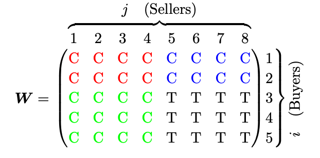
- The outcome is observable at the pair level, and the intervention can occur at the pair level (e.g., a strategy acting on a specific creator-user pair).
- Advantages:
- In the absence of spillover effects, it measures ATE with higher validity.
- When spillover and network interference are present, they can be measured.
- It can be adjusted or extended to measure more complex spillover or interference effects.
-
-
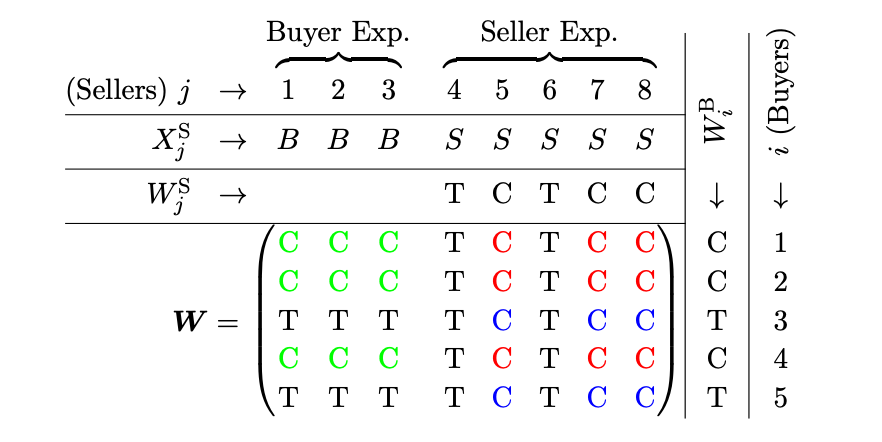
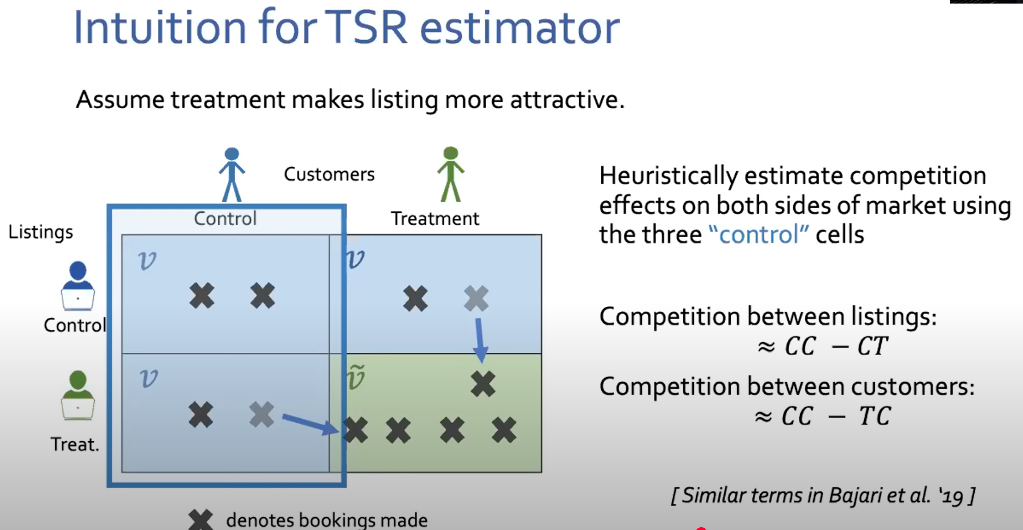
- TSR (Time-Split Randomized) is a special case of MRD.
- It still cannot tell us the true effect of rolling out the strategy to the entire population. However, under the local interference assumption (each pair is only affected by pairs in the same row/column, unaffected by others), it can measure marketplace squeeze. The difference between blue, green, and red can be viewed as the spillover or squeeze effect of the strategy.
- Advantages:
- Similar ideas can be extended to many scenarios:
- For example, in an e-commerce creator support user experiment:
- The difference between treatment and control in the creator treatment group = loss caused by the support strategy.
- The difference between creator treatment and control in the traffic blank group = gains brought by creator behavior (e.g., increased effort, supply).
- The difference between treatment and control in the creator blank group = squeeze effect on active users.
- For example, in an e-commerce creator support user experiment:
- Sometimes double-sided isolation is superimposed:
- For example, Kuaishou Cold Start: restricting a subset of cold-start items to run only on a subset of traffic, isolating the model spillover effect caused by shared samples.
- Reference: Zikun Ye, Dennis J. Zhang, Heng Zhang, Renyu Zhang, Xin Chen, Zhiwei Xu (2023), Cold Start to Improve Market Thickness on Online Advertising Platforms: Data-Driven Algorithms and Field Experiments. Management Science 69(7):3838-3860.
-
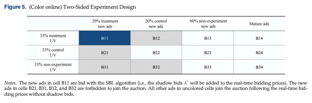
- For example, Kuaishou Cold Start: restricting a subset of cold-start items to run only on a subset of traffic, isolating the model spillover effect caused by shared samples.
Interference (Spillover/Network Interference Between Units)
In standard A/B testing, we rely on the Stable Unit Treatment Value Assumption (SUTVA)—the potential outcome of any unit depends only on the treatment assigned to that unit, independent of the assignments of other units. However, in many practical scenarios, this assumption is violated, causing interference bias.
Interference bias is very common in:
- Social Networks: A user’s behavior is influenced by their friends (e.g., if a friend receives a feature that increases their activity, they might interact more with the user, increasing the user’s activity even if the user is in the control group).
- Shared Resource Markets / Two-Sided Marketplaces: Units compete for shared resources (e.g., ad budgets, ride-hailing drivers, e-commerce buyers). If treatment ads bid more aggressively, they will squeeze out control ads, leading to an overestimation of the treatment effect.
Direct Interference between Units
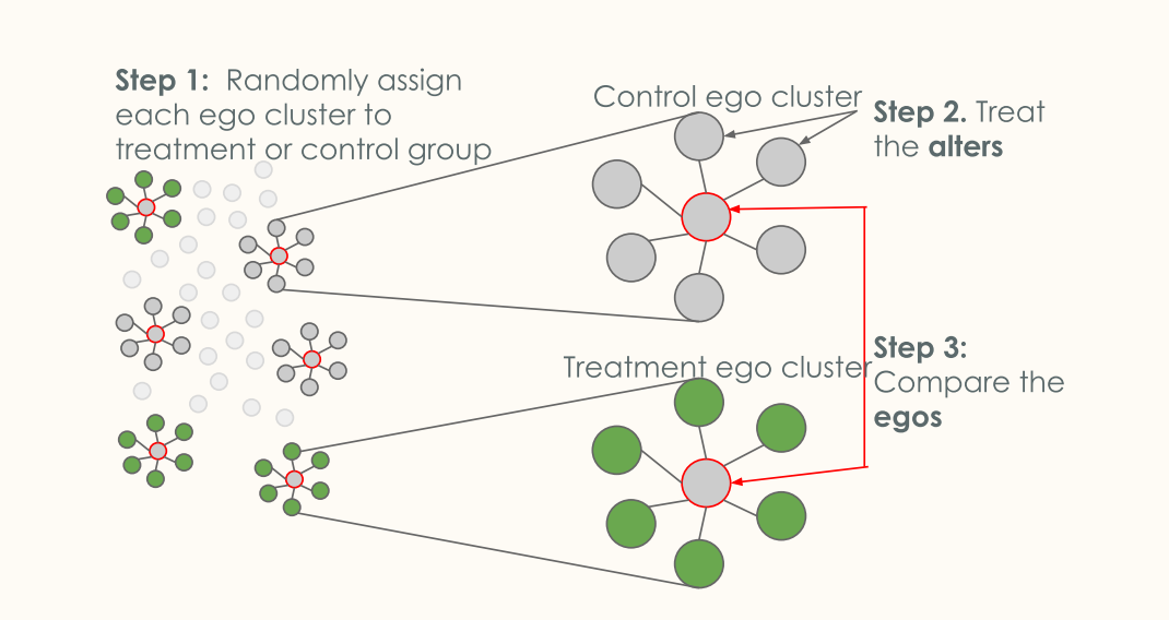
In social networks, direct interference occurs when users interact.
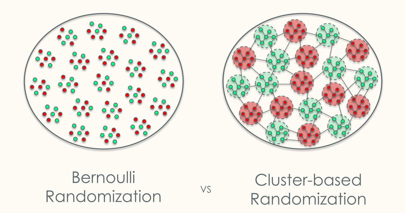
- Solution: Cluster-based Randomized Design (CRD)
- Detect community structures in the network and partition the network into clusters.
- Randomly assign entire clusters to either treatment or control.
- This ensures that most interactions occur within the same group, reducing spillover across groups.
-
-
Indirect Interference: Two-Sided Marketplace
In two-sided marketplaces (e.g., Uber/Lyft, Airbnb, ad auctions), units interfere with each other indirectly through market mechanisms (competition for supply or demand).
Solution 1: Social Network Clustering / Physical Isolation
- Grouping units based on social connections or geographical locations (e.g., partitioning by city) and assigning entire cities/regions to treatment or control.
- Pros: Minimizes spillover.
- Cons: Limited number of cities/clusters leads to high variance and low statistical power.
Solution 2: Time Isolation / Switchback Experiments
- Partitioning the marketplace by time intervals (e.g., 30-minute windows) and switching the entire market between treatment and control states.
-
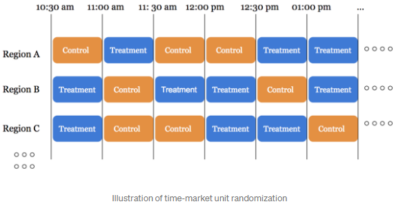
- Pros: Simple to implement; preserves the overall market state.
- Cons: Prone to carryover effects (the effect of the strategy in one time window spills into the next). Requires optimal window length selection to balance carryover bias and variance.
Solution 3: Double-Sided Experiments
- Assigning both sides of the market (e.g., both buyers and sellers, or ads and users) to treatment and control.
- TSR (Time-Split Randomized) and MRD (Multiple Randomization Designs) are common frameworks for this.
-
Reference
- Xu Jia, Causal Inference Challenges in Industry, A perspective from experiences at LinkedIn; Talk
- Lassen, et al., 2022. Statistical Challenges in Online Controlled Experiments: A Review of A/B Testing Methodology
- Johnson, G. A. (2020, April 20). Inferno: A guide to field experiments in online display advertising.
- Patrick Bajari, Brian Burdick, Guido W. Imbens, Lorenzo Masoero, James McQueen, Thomas Richardson, Ido M. Rosen, 2021. Multiple Randomization Designs
- Ramesh Johari, Hannah Li, Inessa Liskovich, Gabriel Weintraub, 2020. Experimental Design in Two-Sided Platforms: An Analysis of Bias
- Li, et al. Interference, Bias, and Variance in Two-Sided Marketplace Experimentation: Guidance for Platforms
- David Holtz, Ruben Lobel, Inessa Liskovich, Sinan Aral, 2020. Reducing Interference Bias in Online Marketplace Pricing Experiments